1.2 Displaying Distributions with Graphs
For each variable, the cases generally will have different values. The distribution of a variable describes how the values of a variable vary from case to case. We can use graphical and numerical descriptions for a distribution. In this section, we start with graphical summaries; we consider numerical summaries in the following section.
Statistical tools and ideas help us examine data to describe their main features. This examination is called exploratory data analysis. Like an explorer crossing unknown lands, we want first to simply describe what we see. Here are two basic strategies that help us organize our exploration of a set of data:
- Begin by examining each variable by itself. Then move on to study the relationships among the variables.
- Begin with a graph or graphs. Then add numerical summaries of specific aspects of the data.
We will follow these principles in organizing our learning. This chapter presents methods for describing a single variable. We will study relationships among several variables in Chapter 2. Within each chapter, we will begin with graphical displays and add numerical summaries for a more complete description.
When we perform an exploratory data analysis, our focus is on a careful description of the values of the variables in our data set. In many applications, particularly in business and economics, our real interest is in using our descriptions to predict something in the future. We use the term predictive analytics to describe data used in this way.
For example, if Trader Joe’s wanted to use data to decide where to open a new store, the company might analyze data from its current stores with a focus on characteristics of stores that are very successful. If managers can find a new location with characteristics that are similar, they would predict that a new store in that location will be successful.
Categorical variables: Bar graphs and pie charts
The values of a categorical variable are names for the categories, such as “yes” and “no.” The distribution of a categorical variable lists the categories and gives either the count or the percent of cases that fall in each category. An alternative to the percent is the proportion, the count divided by the sum of the counts. Note that the percent is simply the proportion times 100.
Example 1.6 Choosing a credit card.
![]()

In a study, 1659 U.S. adults were asked about their reasons for choosing a credit card. Here are the most important reasons that they gave for making their choice.4
| Reason |
Count
|
|---|---|
| Cash back | 680 |
| Rewards | 448 |
| Interest rate | 200 |
| Easy to get | 149 |
| Brand | 133 |
| Other | 49 |
| Total | 1659 |
Reason is the categorical variable in this example, and the values are the six different reasons given for the choice.
Note that the last value of the variable Reason is Other, which
includes all other most important reasons not reported here. For data
sets that have a large number of values for a categorical variable, we
often create a category such as this that combines categories with
relatively small counts or percents.
![]() Careful judgment is needed when doing this. You don’t want to cover
up some important piece of information contained in the data by
combining data in this way.
Careful judgment is needed when doing this. You don’t want to cover
up some important piece of information contained in the data by
combining data in this way.
Example 1.7 Reasons as percents.
![]()
When we look at the reasons for choosing a credit card, we see that cash back is the clear winner. As shown in the data set, 680 adults reported cash back as their most important reason for choosing a credit card. To interpret this number, we need to know that the total number of adults surveyed was 1659. When we say that cash back is the winner, we can describe this win by saying that 41% (680 divided by 1659) of the adults reported cash back as their most important reason. Here is a table of the percents for the different reasons:
| Reason | Percent (%) |
|---|---|
| Cash back | 41 |
| Rewards | 27 |
| Interest rate | 12 |
| Easy to get | 9 |
| Brand | 8 |
| Other | 3 |
| Total | 100 |
The use of graphical methods allows us to see this information and other characteristics of the data easily. We now examine two types of graphs, bar graphs and pie charts.
Example 1.8 Bar graph for the credit card choices data.
![]()
Figure 1.2 displays the credit card choices data using a bar graph. The heights of the six bars show the percents of adults who reported each of the reasons for choosing a credit card as their most important factor.
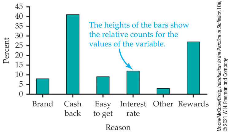
Figure 1.2 Bar graph for the credit card choices data, Example 1.8.
The categories in a bar graph (or pie chart) can be put in any order. In Figure 1.2, we ordered the favorite choices alphabetically. You should always consider the best way to order the values of the categorical variable in a bar graph. Choose an ordering that will be useful to you. If you have difficulty deciding, ask a friend if your choice communicates the message that you expect it to convey. You could also use counts in place of percents. A pie chart, as we’ll see next, naturally uses percents.
Example 1.9 Pie chart for the credit card choices data.
![]()
The pie chart in Figure 1.3 helps us see which part of the whole each group forms. Here it is very easy to see that cash back is the most important reason for about 41% of the adults.
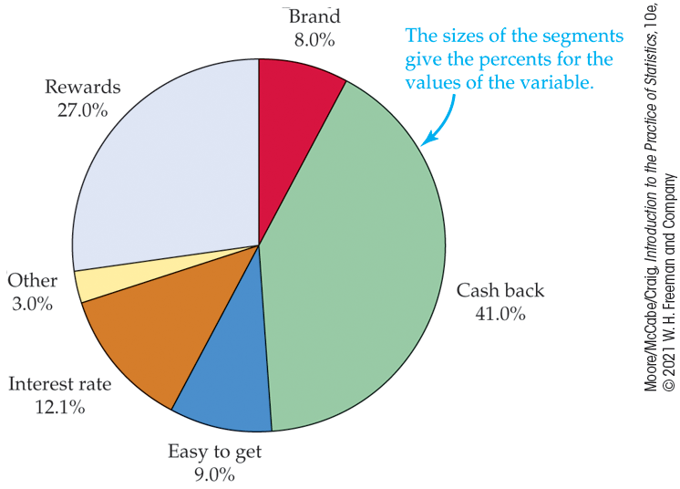
Figure 1.3 Pie chart for the credit card choices data, Example 1.9.
Check-in
-
1.7 Compare the bar graph with the pie chart. Refer to the bar graph in Figure 1.2 and the pie chart in Figure 1.3 for the credit card choices data. Which graphical display does a better job of describing the data? Give reasons for your answer.
Quantitative variables: Stemplots and histograms
A stemplot (also called a stem-and-leaf plot) gives a quick picture of the shape of a distribution while including the actual numerical values in the graph. Stemplots work best for small numbers of observations that are all greater than 0.
Example 1.10 Soluble corn fiber and calcium.
![]()
Soluble corn fiber (SCF) has been promoted for various health benefits. One study examined the effect of SCF on the absorption of calcium of adolescent boys and girls. Calcium absorption is expressed as a percent of calcium in the diet. Here are the data for the condition where subjects consumed 12 grams per day (g/d) of SCF.5
| 50 | 43 | 43 | 44 | 50 | 44 | 35 | 49 | 54 | 76 | 31 | 48 |
| 61 | 70 | 62 | 47 | 42 | 45 | 43 | 59 | 53 | 53 | 73 |
To make a stemplot of these data, use the first digits as stems and the second digits as leaves. Figure 1.4 shows the steps in making the plot, We use the first digit of each value as the stem. Figure 1.4(a) shows the stems that have values 3, 4, 5, 6, and 7. The first entry in our data set is 50. This appears in Figure 1.4(b) on the 5 stem with a leaf of 0. Similarly, the second value, 43, appears in the 4 stem with a leaf of 3. The stemplot is completed in Figure 1.4(c), where the leaves in each row are ordered from smallest to largest.
The middle of the distribution appears to be in the 40s, and the data are more stretched out toward high values than low values. (The highest value is 76, while the lowest is 31.) In the plot, we do not see any extreme values that lie far from the remaining data.
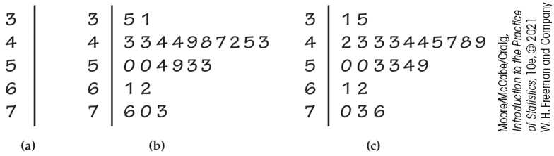
Figure 1.4 Making a stemplot of the data in Example 1.10. (a) Write the stems. (b) Go through the data and write each leaf on the proper stem. For example, the values on the 3 stem are 35 and 31 in the order given in the display for the example. (c) Arrange the leaves on each stem in order out from the stem. The 3 stem now has leaves 1 and 5.
Check-in
-
1.8 Make a stemplot. Here are the scores on the first exam in an introductory statistics course for 28 students in one section of the course:

73 92 82 75 98 94 57 80 90 92 80 87 91 65 70 85 83 61 70 90 75 75 59 68 85 78 80 94 Use these data to make a stemplot. Then use the stemplot to describe the distribution of the first-exam scores for this course.
When you wish to compare two related distributions, a back-to-back stemplot with common stems is useful. The leaves on each side are ordered out from the common stem.
Example 1.11 Soluble corn fiber and calcium.
![]()
Refer to Example 1.10, which gives the data for subjects consuming 12 g/d of SCF. Here are the data for subjects under control conditions (0 g/d of SCF):
| 42 | 33 | 41 | 49 | 42 | 47 | 48 | 47 | 53 | 72 | 47 | 63 |
| 68 | 59 | 35 | 46 | 43 | 55 | 38 | 49 | 51 | 51 | 66 |
Figure 1.5 gives the back-to-back stemplot for the SCF and control conditions. The values on the left give absorption for the control condition, while the values on the right give absorption when SCF was consumed. The values for SCF appear to be somewhat higher than the controls.
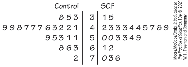
Figure 1.5 A back-to-back stemplot to compare the distributions of calcium absorption under control and SCF conditions, Example 1.11.
Two modifications of the basic stemplot can be helpful in different situations. You can double the number of stems in a plot by splitting stems: separating each stem into two, one with leaves 0 to 4 and the other with leaves 5 through 9. When the observed values have many digits, you can simplify the plot by trimming the numbers, removing the last digit or digits before making a stemplot. If you are using software, you can also round the numbers, which is what was done for the data given in Example 1.11.
You must use your judgment in deciding whether to split stems and whether to trim or round, though statistical software will often make these choices for you. Remember that the purpose of a stemplot is to display the shape of a distribution. If there are many stems with no leaves or only one leaf, trimming will reduce the number of stems. Let’s take a look at the effect of splitting the stems for our SCF data.
Example 1.12 Stemplot with split stems for SCF.
![]()
Figure 1.6 presents the data from Example 1.11 in a stemplot with split stems.
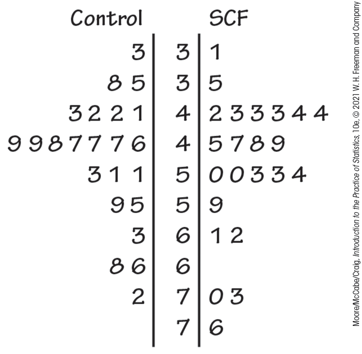
Figure 1.6 A back-to-back stemplot with split stems to compare the distributions of calcium absorption under control and SCF conditions, Example 1.12.
Check-in
-
1.9 Which stemplot do you prefer? Look carefully at the stemplots for the SCF data in Figures 1.5 and 1.6. Which do you prefer? Give reasons for your answer.
-
1.10 Why should you keep the space? Suppose that you had a data set similar to the one given in Example 1.11, but in which the control values of 66 and 68 were both changed to 64.
-
Make a stemplot of these data using split stems.
-
Should you use one stem or two stems for the 60s? Give a reason for your answer. (Hint: How would your choice reveal or conceal a potentially important characteristic of the data?)
-
Histograms
Stemplots display the actual values of the observations. This feature makes stemplots awkward for large data sets. Moreover, the picture presented by a stemplot divides the observations into groups (stems) determined by our base 10 number system rather than by judgment.
Histograms do not have these limitations. A histogram breaks the range of values of a variable into classes and displays only the count or percent of the observations that fall into each class. You can choose any convenient number of classes, but you should choose classes of equal width.
Making a histogram by hand requires more work than a stemplot. In addition, histograms do not display the actual values observed. For these reasons, we prefer stemplots for small data sets.
The construction of a histogram is best shown by example. Most statistical software packages will make a histogram for you.
Example 1.13 Distribution of IQ scores.
![]()
You have probably heard that the distribution of scores on IQ tests is supposed to be roughly “bell-shaped.” Let’s look at some actual IQ scores. Table 1.1 displays the IQ scores of 60 fifth-grade students chosen at random from one school.
| 145 | 139 | 126 | 122 | 125 | 130 | 96 | 110 | 118 | 118 |
| 101 | 142 | 134 | 124 | 112 | 109 | 134 | 113 | 81 | 113 |
| 123 | 94 | 100 | 136 | 109 | 131 | 117 | 110 | 127 | 124 |
| 106 | 124 | 115 | 133 | 116 | 102 | 127 | 117 | 109 | 137 |
| 117 | 90 | 103 | 114 | 139 | 101 | 122 | 105 | 97 | 89 |
| 102 | 108 | 110 | 128 | 114 | 112 | 114 | 102 | 82 | 101 |
To construct a histogram, we proceed as follows:
-
Divide the range of the data into classes of equal width. The classes should be defined so that each score is in exactly one class. Let’s use
Note that a student with IQ 84 would fall into the first class, but IQ 85 is in the second.
-
Count the number of individuals in each class. Each count is called a frequency, and a table of frequencies for all classes is a frequency table.
Class Count Class Count 2 13 3 10 10 5 16 1 -
Draw the histogram. First, on the horizontal axis mark the scale for the variable whose distribution you are displaying—in this case, the IQ score. The scale runs from 75 to 155 because that is the span of the classes we chose. The vertical axis contains the scale of counts. Each bar represents a class. The base of the bar covers the class, and the bar height is the class count. There is no horizontal space between the bars unless a class is empty, so that its bar has height zero. Figure 1.7 is our histogram. It does look roughly “bell-shaped.”
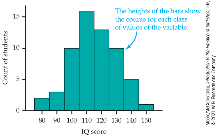
Figure 1.7 Histogram of the IQ scores of 60 fifth-grade students, Example 1.13.
Large sets of data are often reported in the form of frequency tables when it is not practical to publish the individual observations. In addition to the frequency (count) for each class, we may be interested in the fraction or percent of the observations that fall in each class. A histogram of percents looks just like a frequency histogram such as Figure 1.7. Simply relabel the vertical scale to read in percents. Use histograms of percents for comparing several distributions that have different numbers of observations.
Check-in
-
1.11 Make a histogram. Refer to the first-exam scores from Check-in question 1.8 (page 13). Use these data to make a histogram with classes 50 to 59, 60 to 69, etc. Compare the histogram with the stemplot as a way of describing this distribution. Which do you prefer for these data?
Our eyes respond to the area of the bars in a histogram. Because the classes are all the same width, area is determined by height, and all classes are fairly represented. There is no one right choice of the classes in a histogram. Too few classes will give a “skyscraper” graph, with all the values in a few classes with tall bars. Too many will produce a “pancake” graph, with most classes having one or no observations. Neither choice will give a good picture of the shape of the distribution. You must use your judgment in choosing classes to display the shape. Statistical software will choose the classes for you. The software’s choice is often a good one, but you can change it if you want.
![]() You should be aware that the appearance of a histogram can change
when you change the classes.
The histogram function in the
One-Variable Statistical Calculator applet on the text website
allows you to change the number of classes so that it is easy to see
how the choice of classes affects the histogram.
You should be aware that the appearance of a histogram can change
when you change the classes.
The histogram function in the
One-Variable Statistical Calculator applet on the text website
allows you to change the number of classes so that it is easy to see
how the choice of classes affects the histogram.
![]()
Check-in
-
1.12 Change the classes in the histogram. Refer to the first-exam scores from Check-in question 1.8 (page 13) and the histogram that you produced in Check-in question 1.11. Now make a histogram for these data using classes 40 to 59, 60 to 79, and 80 to 100. Compare this histogram with the one that you produced in Check-in question 1.11. Which do you prefer? Give a reason for your answer.
-
1.13 Use smaller classes. Repeat the previous Check-in question using classes 55 to 59, 60 to 64, 65 to 69, etc. Of the three histograms, which do you prefer? Give reasons for your answer.
Although histograms resemble bar graphs, their details and uses are distinct. A histogram shows the distribution of counts or percents among the values of a single quantitative variable. The classes define a range of values, and the heights of the bars represent counts of values within the given range. A bar graph, on the other hand, compares the counts or percents of different values for a single categorical variable. The horizontal axis of a bar graph need not have any measurement scale but may simply identify the values of the categorical variable.
Draw bar graphs with blank space between the bars to separate the
items being compared. Draw histograms with no space to indicate that
all values of the variable are covered.
![]() Some spreadsheet programs, which are not primarily intended for
statistics, will draw histograms as if they were bar graphs, with
space between the bars.
Often, you can tell the software to eliminate the space to produce a
proper histogram.
Some spreadsheet programs, which are not primarily intended for
statistics, will draw histograms as if they were bar graphs, with
space between the bars.
Often, you can tell the software to eliminate the space to produce a
proper histogram.
Examining distributions
Making a statistical graph is not an end in itself. The purpose of the graph is to help us understand the data. After you make a graph, always ask, “What do I see?” Once you have displayed a distribution, you can see its important features as follows.
In Section 1.3, we will learn how to describe center and spread numerically. For now, we can describe the center of a distribution by its midpoint, the value with roughly half the observations taking smaller values and half taking larger values. We can describe the spread of a distribution by giving the smallest and largest values. Stemplots and histograms display the shape of a distribution in the same way. Just imagine a stemplot turned on its side so that the larger values lie to the right.
The extreme values of a distribution are in a tail of the distribution. The high values are in the upper, or right, tail, and the low values are in the lower, or left, tail. Some things to look for in describing shape are
-
Does the distribution have one or several major peaks, each called a mode? A distribution with one major peak is called unimodal. A distribution with two peaks is called bimodal, and a distribution with three peaks is called trimodal.
-
Is it approximately symmetric, or is it skewed in one direction? A distribution is symmetric if the patterns of values smaller and larger than its midpoint are mirror images of each other. It is skewed to the right if the right tail (larger values) is much longer than the left tail (smaller values).
Some variables commonly have distributions with predictable shapes. Many biological measurements on specimens from the same species and sex—lengths of bird bills, heights of young women—have symmetric distributions. Money amounts, on the other hand, usually have right-skewed distributions. There are many moderately priced houses, for example, but the few very expensive mansions give the distribution of house prices a strong right-skew. For small data sets, it is sometimes difficult to see a clear type of shape.
Example 1.14 Examine the histogram of IQ scores.
What does the histogram of IQ scores (Figure 1.7, page 15) tell us?
Shape: The distribution is roughly symmetric, with a single peak in the center. We don’t expect real data to be perfectly symmetric, so in judging symmetry, we are satisfied if the two sides of the histogram are roughly similar in shape and extent.
Center: You can see from the histogram that the midpoint is not far from 110. Looking at the actual data shows that the midpoint is 114.
Spread: The histogram has a spread from 75 to 155. Looking at the actual data shows that the spread is from 81 to 145. There are no outliers or other strong deviations from the symmetric, unimodal pattern.
Check-in
-
1.14 Describe the first-exam scores. Refer to the first-exam scores from Check-in question 1.8 (page 13). Use your favorite graphical display to describe the shape, the center, and the spread of these data. Are there any outliers?
Dealing with outliers
You can spot outliers by looking for observations that stand apart
(either high or low) from the overall pattern of a histogram or
stemplot.
![]() Identifying outliers is a matter for judgment. Look for points that
are clearly apart from the body of the data, not just the most
extreme observations in a distribution. You should search for an
explanation for any outlier.
Sometimes outliers point to errors made in recording the data. In
other cases, the outlying observation may be caused by equipment
failure or other unusual circumstances that would require corrective
action. Outliers can be one of the most important characteristics of a
data set.
Identifying outliers is a matter for judgment. Look for points that
are clearly apart from the body of the data, not just the most
extreme observations in a distribution. You should search for an
explanation for any outlier.
Sometimes outliers point to errors made in recording the data. In
other cases, the outlying observation may be caused by equipment
failure or other unusual circumstances that would require corrective
action. Outliers can be one of the most important characteristics of a
data set.
Example 1.15 College students.
![]()
How does the number of undergraduate college students vary by state? Figure 1.8 is a histogram of the numbers of undergraduate students in each of the states.6 Notice that 52% of the states are included in the first bar of the histogram. These states have fewer than 250,000 undergraduates. The next bar includes another 34% of the states. These have between 250,000 and 500,000 students. The bar at the far right of the histogram corresponds to the state of California, which has 2,415,337 undergraduates. California certainly stands apart from the other states for this variable. It is an outlier.
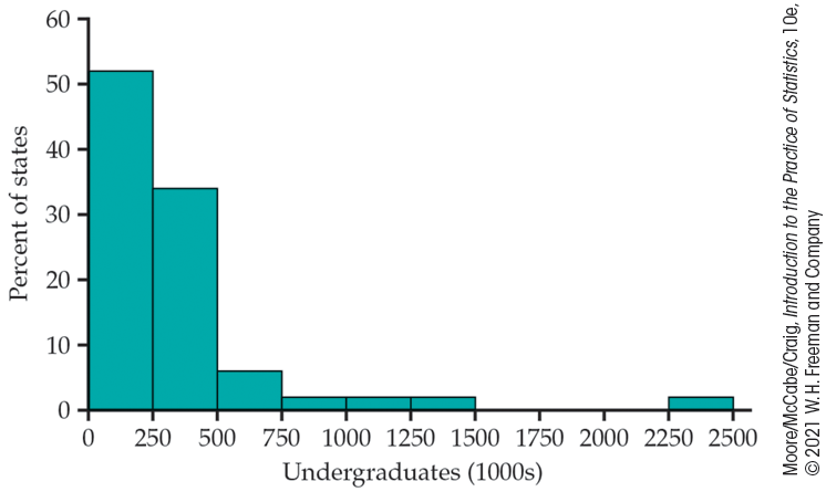
Figure 1.8 The distribution of the numbers of undergraduate college students for the 50 states, Example 1.15.
The state of California is an outlier in Example 1.15 because it has a very large number of undergraduate students. California has the largest population of all the states, so we might expect it to have a large number of college students. Let’s look at these data in a different way.
Example 1.16 College students per 1000.
![]()
To account for the fact that there is large variation in the populations of the states, for each state we divide the number of undergraduate students by the population and then multiply by 1000. This gives the undergraduate college enrollment expressed as the number of students per 1000 people in each state. Figure 1.9 gives a histogram of the distribution. California has 62 undergraduate students per 1000 people. This is one of the higher values in the distribution, but it is clearly not an outlier.
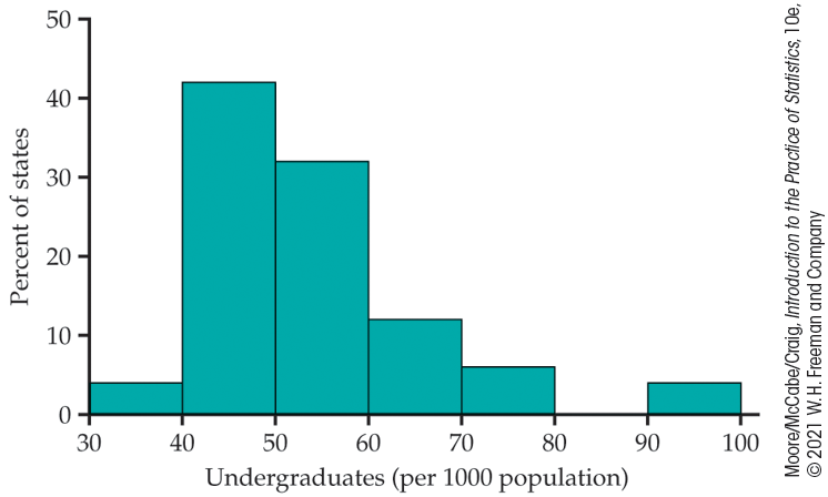
Figure 1.9 The distribution of the numbers of undergraduate college students per 1000 people in each of the 50 states, Example 1.16.
Check-in
-
1.15 Four states with large populations. There are four states with populations greater than 15 million.

-
Examine the data file and report the names of these four states.
-
Find these states in the distribution of number of undergraduate students per 1000 people. To what extent do these four states influence the distribution of number of undergraduate students per 1000 people?
-
In Example 1.15, we looked at the distribution of the number of undergraduate students, while in Example 1.16, we adjusted these data by expressing the counts as number per 1000 people in each state. Which way is correct? The answer depends upon why you are examining the data.
If you are interested in marketing a product to undergraduate
students, the unadjusted numbers would be of interest because you want
to reach the most people. On the other hand, if you are interested in
comparing states with respect to how well they provide opportunities
for higher education to their residents, the population-adjusted
values would be more suitable.
![]() Always think about why you are doing a statistical analysis, and
this will guide you in choosing an appropriate analytic strategy.
Always think about why you are doing a statistical analysis, and
this will guide you in choosing an appropriate analytic strategy.
Here is an example with a different kind of outlier.
Example 1.17 Healthy bones and PTH.
![]()
Bones are constantly being built up (bone formation) and torn down (bone resorption). Young people who are growing have more formation than resorption. When we age, resorption increases to the point where it exceeds formation. (The same phenomenon occurs when astronauts travel in space.) The result is osteoporosis, a disease associated with fragile bones that are more likely to break. The underlying mechanisms that control these processes are complex and involve a variety of substances. One of these is parathyroid hormone (PTH). Here are the values of PTH measured on a sample of 29 boys and girls aged 12 to 15 years:7
| 39 | 59 | 30 | 48 | 71 | 31 | 25 | 31 | 71 | 50 | 38 | 63 | 49 | 45 | 31 |
| 33 | 28 | 40 | 127 | 49 | 59 | 50 | 64 | 28 | 46 | 35 | 28 | 19 | 29 |
The data are measured in picograms per milliliter (pg/ml) of blood. The original data were recorded with one digit after the decimal point. They have been rounded to simplify our presentation here. Figure 1.10 gives a stemplot of the data.
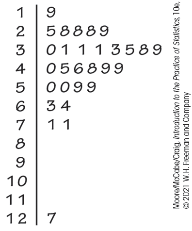
Figure 1.10 Stemplot of the values of PTH, Example 1.17.
The observation 127 clearly stands out from the rest of the distribution. A PTH measurement on this individual taken on a different day was similar to the rest of the values in the data set. We conclude that this outlier was caused by a laboratory error or a recording error, and we are confident in discarding it for any additional analysis.
Time plots
Whenever data are collected over time, it is a good idea to plot the
observations in time order.
![]() Displays of the distribution of a variable that ignore time order,
such as stemplots and histograms, can be misleading when there is
systematic change over time.
Displays of the distribution of a variable that ignore time order,
such as stemplots and histograms, can be misleading when there is
systematic change over time.
Example 1.18 Daily high temperatures in West Lafayette, Indiana.
![]()
In the Northern Hemisphere, temperatures are generally lower during the winter months and higher during the summer months. Figure 1.11 is a plot of the daily high temperatures in West Lafayette, Indiana, for a recent year.8 The temperatures are measured in degrees Fahrenheit, and the days are numbered from 1 to 365, corresponding to January 1 and December 31, respectively. Starting with day 1, the pattern increases, then levels off around day 150 to 250, and then decreases for the remaining days.
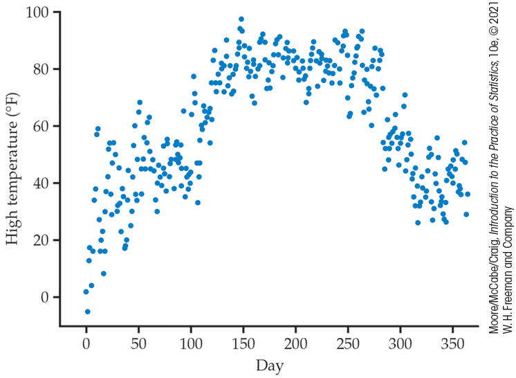
Figure 1.11 Plot of high temperature versus day of the year in West Lafayette, Indiana for a recent year, Example 1.18.
The general pattern we see in Figure 1.11 is expected, but the plot gives us additional information about the temperatures. The summer high temperatures are around 80°F, and January is the coldest month, somewhat colder than December. Although there is a clear overall pattern, there is considerable variation around it, with a range of about 20°F.
Plots of variables measured over time can reveal important facts that need to be taken into account in drawing conclusions from data. The changes in daily high temperature throughout the year are associated with the numbers of hours of daylight. Cells in the skin make vitamin D in response to sunlight. As a result, blood serum levels of vitamin D tend to be lower in winter months, particularly for people who live in northern areas. An analysis of serum vitamin D levels that does not account for the time of year can be very misleading.
Section 1.2 SUMMARY
-
Exploratory data analysis uses graphs and numerical summaries to describe the variables in a data set and the relations among them.
-
The distribution of a variable tells us what values it takes and how often it takes these values.
-
To describe a distribution, begin with a graph. Bar graphs and pie charts display the distribution of a categorical variable. Stemplots and histograms display the distributions of a quantitative variable.
-
When examining any graph, look for an overall pattern and for clear deviations from that pattern.
-
Shape, center, and spread describe the overall pattern of a distribution. Some distributions have simple shapes, such as symmetric or skewed. Not all distributions have a simple overall shape, especially when there are few observations.
-
Outliers are observations that lie outside the overall pattern of a distribution. Always look for outliers and try to explain them.
-
When observations on a variable are taken over time, make a time plot that graphs time horizontally and the values of the variable vertically. A time plot can reveal interesting patterns in a set of data.
Section 1.2 EXERCISES
-
1.10 What’s wrong? Explain what is wrong with each of the following:
-
A stemplot can be used to display the distribution of a categorical variable.
-
A symmetric distribution can be skewed to the right.
-
Always discard outliers before doing an analysis of a set of data.
-
-
1.11 Which graphical display should you use? For each of the following scenarios, decide which graphical display (pie chart, bar graph, stemplot, or histogram) you would use to describe the distribution of the variable. Give a reason for your choice and, if there is an alternative choice that would also be reasonable, explain why your choice was better than the alternative.
-
The number of minutes you spent sleeping on each of the seven days in the past week.
-
The grades on the first exam in a statistics course for the 120 students enrolled in the course
-
The favorite color of each student in the statistics course
-
The number of students in the graduating high school class for each high school in Iowa
-
-
1.12 Frequent users of social media. A recent survey by the Pew Research Center asked social media users about how often they visited various sites. Pew defined a frequent user to be someone who visited a site several times a day. Here are the percents of users who are frequent users for several popular sites:9

Social media Frequent users (%) Facebook 51 Snapchat 46 Instagram 42 YouTube 32 Twitter 25 Use a bar graph to describe the percents of frequent users of these sites and write a short summary of the data based on your graph.
-
1.13 Pie chart for frequent users of social media. Refer to the previous exercise.
-
Use a pie chart to describe the percents of frequent users of these sites and write a short summary of the data based on your chart.
-
Compare this pie chart with the bar graph that you produced for the previous exercise. Which do you prefer? Give reasons for your answer.
-
-
1.14 Facebook users by country. The following table gives the numbers of active Facebook users by country for the top 11 countries based on the number of users in July 2019.10

Country Facebook users
(in millions)India 270 United States 190 Indonesia 130 Brazil 120 Mexico 82 Philippines 68 Vietnam 58 Thailand 46 Egypt 38 Turkey 37 United Kingdom 37 -
Use a bar graph to describe the numbers of users in these countries.
-
Describe the major features of your graph in a short paragraph.
-
-
1.15 Potassium from potatoes. The 2015 Dietary Guidelines for Americans11 notes that the average potassium (K) intake for U.S. adults is about half of the recommended amount. A major source of potassium is potatoes. Nutrients in the diet can have different absorption depending on the source. One study looked at absorption of potassium, measured in milligrams (mg), from different sources. Participants ate a controlled diet for five days, and the amount of potassium absorbed was measured. Data for a diet that included 40 milliequivalents (mEq) of potassium were collected from 27 adult subjects.12

-
Make a stemplot of the data.
-
Describe the pattern of the distribution.
-
Are there any outliers? If yes, describe them and explain why you have declared them to be outliers.
-
Describe the shape, center, and spread of the distribution.
-
-
1.16 Potassium from a supplement. Refer to the previous exercise. Data were also recorded for 29 subjects who received a potassium salt supplement with 40 mEq of potassium. Answer the questions in the previous exercise for the supplemented subjects.

-
1.17 Energy consumption. The U.S. Energy Information Administration reports data summaries of various energy statistics. Let’s look at the total amount of energy consumed, in quadrillions of British thermal units (Btu), for each month in a recent year. Here are the data:13

Month Energy
(quadrillion Btu)Month Energy
(quadrillion Btu)January 9.58 July 8.23 February 8.46 August 8.21 March 8.56 September 7.64 April 7.56 October 7.78 May 7.66 November 8.19 June 7.79 December 8.82 -
Look at the table and describe how the energy consumption varies from month to month.
-
Make a time plot of the data and describe the patterns.
-
Suppose you wanted to communicate information about the month-to-month variation in energy consumption. Which would be more effective, the table of the data or the graph? Give reasons for your answer.
-
-
1.18 Energy consumption in a different year. Refer to the previous exercise. Here are the data for the previous year:
Month Energy
(quadrillion Btu)Month Energy
(quadrillion Btu)January 8.99 July 8.27 February 8.02 August 8.17 March 8.38 September 7.64 April 7.52 October 7.72 May 7.62 November 8.14 June 7.72 December 9.08 -
Analyze these data using the questions in the previous exercise as a guide.
-
Compare the patterns across the two years. Describe any similarities and differences.
-
-
1.19 Least favorite colors. What is your least favorite color? One survey produced the following summary of responses to that question: brown, 23%; green, 4%; gray, 12%; orange, 30%; other, 1%; purple, 13%; white; 4%; yellow, 13%.14

-
Make a bar graph of the percents with the colors ordered alphabetically as they are given in this exercise.
-
Make a second bar graph with the colors ordered by the percents, largest to smallest. This type of bar graph is called a Pareto chart.
-
Write a short paragraph comparing these two ways to display the data graphically. Which do you prefer? Give a reason for your preference.
-
-
1.20 Cheap colors. Refer to the previous exercise. The same study also asked people about what colors they associate with the words cheap/inexpensive. Here are the results: brown, 13%; green, 6%; gray, 8%; orange, 26%; other, 3%; purple, 4%; red, 9%; white; 9%; yellow, 22%. Answer the questions from the previous exercise for these data.

-
1.21 Garbage. The formal name for garbage is “municipal solid waste.” In the United States, approximately 250 million tons of garbage are generated in a year. Here is a breakdown of the materials that made up American municipal solid waste in a recent year:15

Material Weight
(million tons)Percent of total Food scraps 39.7 15.1 Glass 11.5 4.4 Metals 24.0 9.1 Paper, paperboard 68.0 25.9 Plastics 34.5 13.1 Rubber, leather 8.5 3.2 Textiles 16.0 6.1 Wood 16.3 6.2 Yard trimmings 34.7 13.3 Other 9.2 3.6 Total 262.4 100.0 -
Make a bar graph of the percents. The graph gives a clearer picture of the main contributors to garbage if you order the bars from tallest to shortest, as in a Pareto chart (see Exercise 1.19).
-
Also make a pie chart of the percents.
-
Compare the two graphs. Which do you prefer? Give reasons for your answer.
-
-
1.22 Vehicle colors. Vehicle colors differ among regions of the world. Here are data on the most popular colors for vehicles in North America:16

Color Percent White 24 Black 19 Silver 16 Gray 15 Red 10 Blue 7 Brown 5 Other 4 -
Describe these data with a bar graph.
-
Describe these data with a pie chart.
-
Which graphical summary do you prefer? Give reasons for your answer.
-
-
1.23 Grades and self-concept. Table 1.2 presents data on 78 seventh-grade students in a rural midwestern school.17 The researcher was interested in the relationship between the students’ “self-concept” and their academic performance. The data we give here include each student’s grade point average (GPA), score on a standard IQ test, and sex, taken from school records. Sex is coded as F for female and M for male. The students are identified only by an observation number. The missing observation numbers show that some students dropped out of the study. The final variable is each student’s score on the Piers-Harris Children’s Self-Concept Scale, a psychological test administered by the researcher.

-
How many variables does this data set contain? Which are categorical variables, and which are quantitative variables?
-
Make a histogram of the distribution of GPA.
-
Make a stemplot of the distribution of GPA.
-
Do you prefer the histogram or the stemplot? Explain your choice.
-
Describe the shape, center, and spread of the GPA distribution. Identify any suspected outliers from the overall pattern.
-
Make a back-to-back stemplot of the rounded GPAs for female and male students. Write a brief comparison of the two distributions.
-
-
1.24 Describe the IQ scores. Make a graph of the distribution of IQ scores for the seventh-grade students in Table 1.2. Describe the shape, center, and spread of the distribution, as well as any outliers. IQ scores are usually said to be centered at 100. Is the midpoint for these students close to 100, clearly above, or clearly below?
-
1.25 Sketch a skewed distribution. Sketch a histogram for a distribution that is skewed to the left. Suppose that you and your friends emptied your pockets of coins and recorded the year marked on each coin. The distribution of dates would be skewed to the left. Explain why.
-
1.26 Describe the self-concept scores. Based on a suitable graph, briefly describe the distribution of self-concept scores for the students in Table 1.2. Be sure to identify any suspected outliers.
Table 1.2 Educational data for 78 seventh-grade students
Obs GPA IQ Gender Self Obs GPA IQ Gender Self 001 7.940 111 M 67 043 10.760 123 M 64 002 8.292 107 M 43 044 9.763 124 M 58 003 4.643 100 M 52 045 9.410 126 M 70 004 7.470 107 M 66 046 9.167 116 M 72 005 8.882 114 F 58 047 9.348 127 M 70 006 7.585 115 M 51 048 8.167 119 M 47 007 7.650 111 M 71 050 3.647 97 M 52 008 2.412 97 M 51 051 3.408 86 F 46 009 6.000 100 F 49 052 3.936 102 M 66 010 8.833 112 M 51 053 7.167 110 M 67 011 7.470 104 F 35 054 7.647 120 M 63 012 5.528 89 F 54 055 0.530 103 M 53 013 7.167 104 M 54 056 6.173 115 M 67 014 7.571 102 F 64 057 7.295 93 M 61 015 4.700 91 F 56 058 7.295 72 F 54 016 8.167 114 F 69 059 8.938 111 F 60 017 7.822 114 F 55 060 7.882 103 F 60 018 7.598 103 F 65 061 8.353 123 M 63 019 4.000 106 M 40 062 5.062 79 M 30 020 6.231 105 F 66 063 8.175 119 M 54 021 7.643 113 M 55 064 8.235 110 M 66 022 1.760 109 M 20 065 7.588 110 M 44 024 6.419 108 F 56 068 7.647 107 M 49 026 9.648 113 M 68 069 5.237 74 F 44 027 10.700 130 F 69 071 7.825 105 M 67 028 10.580 128 M 70 072 7.333 112 F 64 029 9.429 128 M 80 074 9.167 105 M 73 030 8.000 118 M 53 076 7.996 110 M 59 031 9.585 113 M 65 077 8.714 107 F 37 032 9.571 120 F 67 078 7.833 103 F 63 033 8.998 132 F 62 079 4.885 77 M 36 034 8.333 111 F 39 080 7.998 98 F 64 035 8.175 124 M 71 083 3.820 90 M 42 036 8.000 127 M 59 084 5.936 96 F 28 037 9.333 128 F 60 085 9.000 112 F 60 038 9.500 136 M 64 086 9.500 112 F 70 039 9.167 106 M 71 087 6.057 114 M 51 040 10.140 118 F 72 088 6.057 93 F 21 041 9.999 119 F 54 089 6.938 106 M 56 -
1.27 The Boston Marathon. Women were allowed to enter the Boston Marathon in 1972. Table 1.3 gives the times (in minutes, rounded to the nearest minute) for the winning women from 1972 to 2019.18
Table 1.3 Boston Marathon winning times for women
Year Time Year Time Year Time Year Time 1972 190 1984 149 1996 147 2008 145 1973 186 1985 154 1997 146 2009 152 1974 167 1986 145 1998 143 2010 146 1975 162 1987 146 1999 143 2011 142 1976 167 1988 145 2000 146 2012 151 1977 168 1989 144 2001 144 2013 146 1978 165 1990 145 2002 141 2014 140 1979 155 1991 144 2003 145 2015 145 1980 154 1992 144 2004 144 2016 149 1981 147 1993 145 2005 145 2017 142 1982 150 1994 142 2006 143 2018 160 1983 143 1995 145 2007 149 2019 144 Make a graph that shows change over time. What overall pattern do you see? Have times stopped improving in recent years? If so, when did improvement end?