1.3 Describing Distributions with Numbers
We can begin our data exploration with graphs, but numerical summaries make our analysis more specific. For categorical variables, numerical summaries are the counts or percents that we use to construct pie charts or bar graphs. In this section, we focus on numerical summaries for quantitative variables. A brief description of the distribution of a quantitative variable should include its shape and numbers describing its center and spread. We describe the shape of a distribution based on inspection of a histogram or a stemplot. Now we will learn specific ways to use numbers to measure the center and spread of a distribution. We can calculate these numerical measures for any quantitative variable. But to interpret measures of center and spread, and to choose among the several measures we will examine, you must think about the shape of the distribution and the meaning of the data. The numbers, like graphs, are aids to understanding, not “the answer” in themselves.
Example 1.19 The distribution of business start times.
![]()
An entrepreneur faces many bureaucratic and legal hurdles when starting a new business. The World Bank collects information about starting businesses throughout the world. It has determined the time, in days, to complete all the procedures required to start a business.19 Data for 187 countries are included in the data set, TTS. For this example, we examine data, rounded to integers, for a sample of 24 of these countries. Here are the data:
| 19 | 17 | 43 | 7 | 12 | 27 | 67 | 49 | 6 | 6 | 29 | 12 |
| 12 | 9 | 17 | 23 | 1 | 12 | 14 | 18 | 6 | 7 | 9 | 31 |
The stemplot in Figure 1.12 shows us the shape, center, and spread of the business start times. The stems are tens of days, and the leaves are days. The distribution is skewed to the right, with a very long tail of high values. All but seven of the times are less than 20 days. The center appears to be about 12 days, and the values range from 1 day to 67 days.
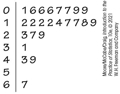
Figure 1.12 Stemplot for the sample of 24 business start times, Example 1.19.
Measuring center: The mean
Numerical description of a distribution begins with a measure of its center or average. The two common measures of center are the mean and the median. The mean is the “average value,” and the median is the “middle value.” These are two different ideas for “center,” and the two measures behave differently. We need precise recipes for the mean and the median.
The ∑ (capital Greek sigma) in the formula for the mean is short for
“add them all up.” The bar over the
Example 1.20 Mean time to start a business.
![]()
The mean time to start a business is
The mean time to start a business for the 24 countries in our data set is 19 days. Note that we have rounded the answer. Our goal in using the mean to describe the center of a distribution is not to demonstrate that we can compute with great accuracy. The additional digits do not provide any additional useful information. In fact, they distract our attention from the important digits that are meaningful. Do you think it would be better to report the mean as 18.9 days?
The value of the mean will not necessarily be equal to the value of one of the observations in the data set. Our example of time to start a business illustrates this fact.
In practice, you can key the data into your calculator and hit the Mean key. You don’t have to actually add and divide. But you should know that this is what the calculator is doing.
Check-in
-
1.16 Include the outlier. For Example 1.19, a random sample of 24 countries was selected from a data set that included 187 countries. The South American country Venezuela, where the start time is 230 days, was not included in the random sample. Consider the effect of adding Venezuela to the original set. Show that the mean for the new sample of 25 countries has increased to 27 days. (This is a rounded number. You should report the mean with two digits after the decimal to show that you have performed this calculation.)

-
1.17 Find the mean. Here are the scores on the first exam in an introductory statistics course for 10 students:

75 87 94 85 74 98 93 52 80 91 Find the mean first-exam score for these students.
Check-in question 1.16
illustrates an important weakness of the mean as a measure of center:
![]() the mean is sensitive to the influence of a few extreme
observations.
These may be outliers, but a skewed distribution that has no outliers
will also pull the mean toward its long tail. Because the mean cannot
resist the influence of extreme observations, we say that it is not a
resistant
measure
of center.
the mean is sensitive to the influence of a few extreme
observations.
These may be outliers, but a skewed distribution that has no outliers
will also pull the mean toward its long tail. Because the mean cannot
resist the influence of extreme observations, we say that it is not a
resistant
measure
of center.
A measure that is resistant does more than limit the influence of outliers. Its value does not respond strongly to changes in a few observations, no matter how large those changes may be. The mean fails this requirement because we can make the mean as large as we wish by making a large enough increase in just one observation. A resistant measure is sometimes called a robust measure.
Measuring center: The median
We used the midpoint of a distribution as an informal measure of center in Section 1.2. The median is the formal version of the midpoint, with a specific rule for calculation.
![]() Note that the formula
Note that the formula
Example 1.21 Median time to start a business.
![]()
To find the median time to start a business for our 24 countries, we first arrange the data in order from smallest to largest:
| 1 | 6 | 6 | 6 | 7 | 7 | 9 | 9 | 12 | 12 | 12 | 12 |
| 14 | 17 | 17 | 18 | 19 | 23 | 27 | 29 | 31 | 43 | 49 | 67 |
The count of observations
Therefore, the center observations are the 12th and 13th observations in the ordered list. The median is
Note that you can use the stemplot in Figure 1.12 (page 26) directly to compute the median. In the stemplot, the cases are already ordered, and you simply need to count from the top or the bottom to the desired location.
Check-in
-
1.18 Where is the median? Suppose that the sample size is 25. Find the location of the median.
-
1.19 Include the outlier. Include Venezuela, where the start time is 230 days, in the data set, and show that the median is 14 days. Write out the ordered list and circle the outlier. Describe the effect of the outlier on the median for this set of data.
-
1.20 Find the median. Here are the scores on the first exam in an introductory statistics course for 10 students:
75 87 94 85 74 98 93 52 80 91 Find the median first-exam score for these students.
Comparing the mean and the median
Check-in questions 1.16 (page 27) and 1.19 (above) illustrate an important difference between the mean and the median. Venezuela is an outlier. It pulls the mean time to start a business up from 19 days to 27 days. The median increased slightly, from 13 days to 14 days.
The median is more resistant than the mean. If the largest start time in the data set were 1200 days, the median for all 25 countries would still be 14 days. The largest observation just counts as one observation above the center, no matter how far above the center it lies. The mean uses the actual value of each observation, and so a single large observation will pull the mean upward.
A good way to compare the responses of the mean and median to extreme
observations is to use an interactive applet that allows you to place
points on a line and then drag them with your computer’s mouse.
Exercises 1.53 and
1.54 use the
Mean and Median applet on the website for this text to compare
the mean and the median.
![]()
The median and mean are the most common measures of the center of a distribution. For a symmetric distribution, they are close together. If a distribution is exactly symmetric, the mean and median are exactly the same. In a skewed distribution, the mean is farther out in the long tail than is the median.
The endowment for a college or university is money set aside and
invested. The income from the endowment is usually used to support
various programs. The distribution of the sizes of the endowments of
colleges and universities is strongly skewed to the right. Most
institutions have modest endowments, but a few are very wealthy. The
median endowment of colleges and universities in a recent year was
$142 million—but the mean endowment was $771 million.20
The few wealthy institutions pull the mean up but do not affect the
median.
![]() Don’t confuse the “average” value of a variable (the mean) with its
“typical” value, which we might describe by the median.
Don’t confuse the “average” value of a variable (the mean) with its
“typical” value, which we might describe by the median.
We can now give a better answer to the question of how to deal with outliers in data. First, look at the data to identify outliers and investigate their causes. You can then correct outliers if they are wrongly recorded, delete them for good reason, or otherwise give them individual attention. The outliers in a data set can be the most important feature of the distribution.
The outlier in Example 1.17 (page 19) can be dropped from the data once we discover that it is an error. If you have no clear reason to drop outliers, you may want to use resistant measures in your analysis so that outliers have little influence over your conclusions. The choice is often a matter for judgment.
Measuring spread: The quartiles
A measure of center alone can be misleading. Two countries with the same median family income are very different if one has extremes of wealth and poverty and the other has little variation among families. A drug manufactured with the correct mean concentration of active ingredient is dangerous if some batches are much too high and others much too low.
We are interested in the spread or variability of incomes and drug potencies as well as their centers. The simplest useful numerical description of a distribution consists of both a measure of center and a measure of spread.
The median divides the data in two; half of the observations are above the median, and half are below the median. The upper quartile is the median of the upper half of the data. Similarly, the lower quartile is the median of the lower half of the data. With the median, the quartiles divide the data into four equal parts; 25% of the data are in each part.
We can do a similar calculation for any percent. The pth percentile of a distribution is the value that has p% of the observations fall at or below it. We could call the median the 50th percentile. To calculate a percentile, arrange the observations in increasing order and count up the required percent from the bottom of the list.
Our definition of percentiles is a bit inexact because there is not always a value with exactly p% of the data at or below it. We will be content to take the nearest observation for most percentiles, but the quartiles are important enough to require an exact rule.
Here is an example that shows how the rules for quartiles work for even numbers of observations.
Example 1.22 Finding the quartiles.
![]()
Here is the ordered list of the times to start a business in our sample of 24 countries:
| 1 | 6 | 6 | 6 | 7 | 7 | 9 | 9 | 12 | 12 | 12 | 12 |
| 14 | 17 | 17 | 18 | 19 | 23 | 27 | 29 | 31 | 43 | 49 | 67 |
The count of observations
Notice that the quartiles are resistant. For example,
![]() Be careful when several observations take the same numerical
value.
Write down all the observations and apply the rules just as if they
all had distinct values.
Be careful when several observations take the same numerical
value.
Write down all the observations and apply the rules just as if they
all had distinct values.
Check-in
-
1.21 Find the quartiles. Here are the scores on the first exam in an introductory statistics course for 10 students:
75 87 94 85 74 98 93 52 80 91 Find the quartiles for these first-exam scores.
![]() There are several rules for calculating quartiles, which often give
slightly different values.
The differences are generally small. For describing data, just report
the values that your software gives.
There are several rules for calculating quartiles, which often give
slightly different values.
The differences are generally small. For describing data, just report
the values that your software gives.
The five-number summary and boxplots
In
Section 1.2, we used the smallest and largest observations to indicate the
spread of a distribution. These single observations tell us little
about the distribution as a whole, but they give information about the
tails of the distribution that is missing if we know only
Example 1.23 The five-number summary for the PTH data.
![]()
Let’s find the five-number summary for the PTH scores in Example 1.17. Here is the ordered list of PTH values for our sample of 29 children, arranged specifically for this summary:
| 19 | 25 | 28 | 28 | 28 | 29 | 30 |
| 31 | 31 | 31 | 33 | 35 | 38 | 39 |
| 40 | ||||||
| 45 | 46 | 48 | 49 | 49 | 50 | 50 |
| 59 | 59 | 63 | 64 | 71 | 71 | 127 |
The sample size is 29, so the median is the located at position
Check-in
-
1.22 Find the five-number summary. Here are the scores on the first exam in an introductory statistics course for 10 students:
75 87 94 85 74 98 93 52 80 91 Find the five-number summary for these first-exam scores.
The five-number summary leads to another visual representation of a distribution, the boxplot.
The lines extending to the smallest and largest observations are sometimes called whiskers, and boxplots are sometimes called box-and-whisker plots. Software provides many varieties of boxplots, some of which use different choices for the placement of the whiskers.
When you look at a boxplot, first locate the median, which marks the center of the distribution. Then look at the spread. The quartiles show the spread of the middle half of the data, and the extremes (the smallest and largest observations) show the spread of the entire data set.
Example 1.24 IQ scores.
![]()
In
Example 1.13
(page 14), we
used a histogram to examine the distribution of a sample of 60 IQ
scores. A boxplot for these data is given in
Figure 1.13. Note that the
mean is marked with a
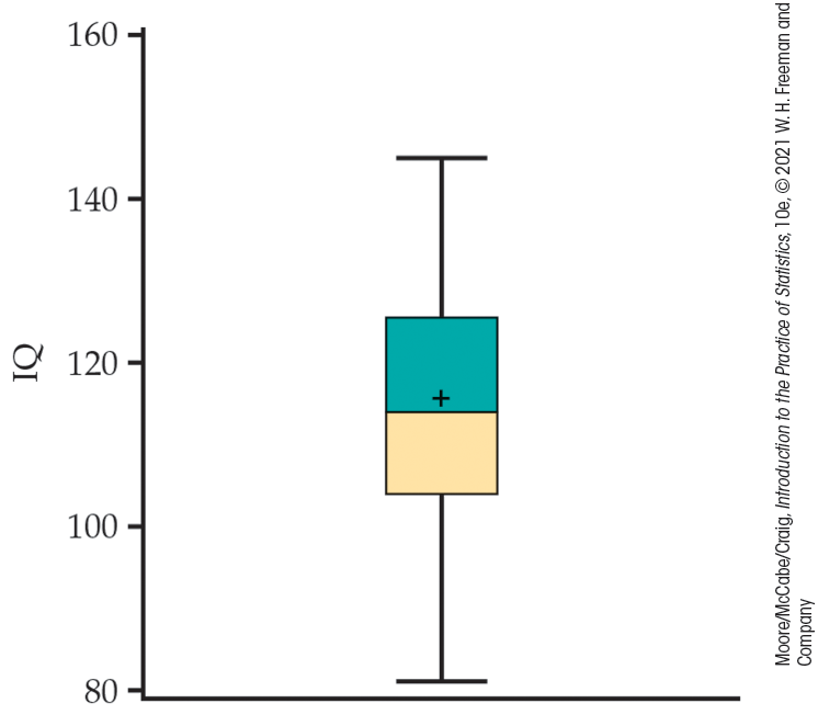
Figure 1.13 Boxplot for sample of 60 IQ scores, Example 1.24.
Check-in
-
1.23 Make a boxplot. Here are the scores on the first exam in an introductory statistics course for 10 students:
75 87 94 85 74 98 93 52 80 91 Make a boxplot for these first-exam scores.
The 1.5 × IQR rule for suspected outliers
If we look at the PTH data in Example 1.17 (page 19), we can spot a clear outlier, a PTH value of 127, which is almost twice as high as the next highest value. How can we describe the spread of this distribution? The smallest and largest observations are extremes that do not describe the spread of the majority of the data. The distance between the quartiles (the range of the center half of the data) is a more resistant measure of spread than the range. This distance is called the interquartile range.
Example 1.25 IQR for the PTH data.
In Example 1.23 (page 31), we found that the five-number summary for the PTH data is 19, 30.5, 40, 54.5, 127. Therefore, we calculate
The quartiles and the IQR are not affected by changes in either tail of the distribution. They are resistant, therefore, because changes in a few data points have no further effect once these points move outside the quartiles.
![]() However,
no single numerical measure of spread, such as IQR, is very
useful for describing skewed distributions.
The two sides of a skewed distribution have different spreads, so one
number can’t summarize them. We can often detect skewness from the
five-number summary by comparing how far the first quartile and the
minimum are from the median (left tail) with how far the third
quartile and the maximum are from the median (right tail). The
interquartile range is mainly used as the basis for a rule of thumb
for identifying suspected outliers.
However,
no single numerical measure of spread, such as IQR, is very
useful for describing skewed distributions.
The two sides of a skewed distribution have different spreads, so one
number can’t summarize them. We can often detect skewness from the
five-number summary by comparing how far the first quartile and the
minimum are from the median (left tail) with how far the third
quartile and the maximum are from the median (right tail). The
interquartile range is mainly used as the basis for a rule of thumb
for identifying suspected outliers.
Example 1.26 Suspected outliers for the PTH data.
![]()
For the PTH data, we have
The first quartile is 30.5, and the third quartile is 54.5, so any
values below
Check-in
-
1.24 Use the IQR rule for outliers. Here are the scores on the first exam in an introductory statistics course for 10 students:
75 87 94 85 74 98 93 52 80 91 Find the interquartile range and use the
Two variations on the basic boxplot can be very useful. The first,
called a
modified
boxplot, uses the
The other variation is to use two or more boxplots in the same graph to compare groups measured on the same variable. These are called side-by-side boxplots. The following example illustrates these two variations.
Example 1.27 Do poets die young?
![]()
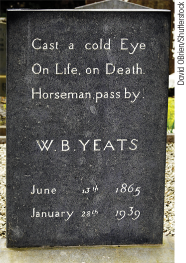
According to William Butler Yeats, “She is the Gaelic muse, for she gives inspiration to those she persecutes. The Gaelic poets die young, for she is restless, and will not let them remain long on earth.” One study designed to investigate this issue examined the age at death for writers from different cultures and genders.21
Three categories of writers examined were novelists, poets, and nonfiction writers. We examine the ages at death for female writers in these categories from North America. Figure 1.14 shows modified side-by-side boxplots for the three categories of writing.
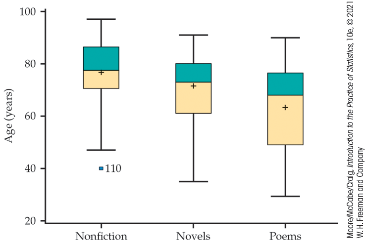
Figure 1.14 Modified side-by-side boxplots for the data on writers’ age at death, Example 1.27.
Displaying the boxplots for the three categories of writing lets us compare the three distributions. We see that nonfiction writers tend to live the longest, followed by novelists. The poets do appear to die young! There is one outlier among the nonfiction writers, which is plotted individually along with the value of its label (110). This writer died at the age of 40, young for a nonfiction writer, but not for a novelist or a poet!
Measuring spread: The standard deviation
![]()
The five-number summary is not the most common numerical description of a distribution. That distinction belongs to the combination of the mean to measure center and the standard deviation to measure spread, or variability. The standard deviation measures spread by looking at how far the observations are from their mean.
The idea behind the variance and the standard deviation as measures of
spread is as follows: The deviations
Example 1.28 Metabolic rate.
![]()
A person’s metabolic rate is the rate at which the body consumes energy. Metabolic rate is important in studies of weight gain, dieting, and exercise. Here are the metabolic rates of seven men who took part in a study of dieting. (The units are calories per 24 hours. These are the same calories used to describe the energy content of foods.)
| 1792 | 1666 | 1362 | 1614 | 1460 | 1867 | 1439 |
Use software to verify that
Figure 1.15 plots these
data as dots on the calorie scale, with their mean marked by an
asterisk
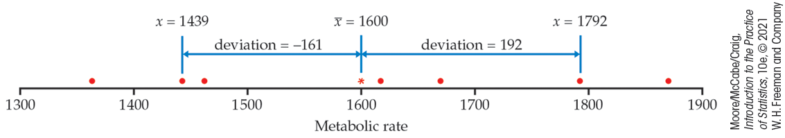
Figure 1.15 Metabolic rates for seven men, with the mean (*) and the deviations of two observations from the mean, Example 1.28.
Exercise 1.52 (page 45) asks you to calculate the seven deviations from
Example 1.28, square
them, and find
Check-in
-
1.25 Find the variance and the standard deviation. Here are the scores on the first exam in an introductory statistics course for 10 students:
75 87 94 85 74 98 93 52 80 91 Find the variance and the standard deviation for these first-exam scores.
The idea of the variance is straightforward: it is the average of the squares of the deviations of the observations from their mean. The details we have just presented, however, raise some questions.
Why do we square the deviations?
-
First, the sum of the squared deviations of any set of observations from their mean is the smallest that the sum of squared deviations from any number can possibly be. This is not true of the unsquared distances. So squared deviations point to the mean as center in a way that other distances do not.
-
Second, the standard deviation turns out to be the natural measure of spread for a particularly important class of symmetric unimodal distributions, the Normal distributions. We will meet the Normal distributions in the next section.
Why do we emphasize the standard deviation rather than the variance?
-
One reason is that
-
There is also a more general reason to prefer
Why do we average by dividing by
-
Because the sum of the deviations is always zero, the last deviation can be found once we know the other
-
The number
Properties of the standard deviation
Here are the basic properties of the standard deviation
Check-in
-
1.26 A standard deviation of zero. Construct a data set with four cases that has a variable with
![]() The use of squared deviations renders
The use of squared deviations renders
Check-in
-
1.27 Effect of an outlier on the IQR. Find the IQR for the time to start a business with and without Venezuela. What do you conclude about the sensitivity of this measure of spread to the inclusion of an outlier?

Choosing measures of center and spread
How do we choose between the five-number summary and
Remember that a graph gives the best overall picture of a
distribution.
![]() Numerical measures of center and spread report specific facts about
a distribution, but they do not describe its shape.
Numerical summaries do not disclose the presence of multiple modes or
gaps, for example. Always plot your data.
Numerical measures of center and spread report specific facts about
a distribution, but they do not describe its shape.
Numerical summaries do not disclose the presence of multiple modes or
gaps, for example. Always plot your data.
Example 1.29 Results from software.
![]()
We prefer to examine the numerical summaries and graphical summaries together. Figure 1.16 gives a boxplot, a histogram, and numerical summaries for the time to start a business data from Example 1.19 (page 26) using Minitab. Similar displays are given for SPSS in Figure 1.17 and for JMP in Figure 1.18. Examine and compare the outputs carefully. Notice that they give different numbers of significant digits for some of these numerical summaries. There are also variations in how they make the boxplots and how they define classes for the histograms.
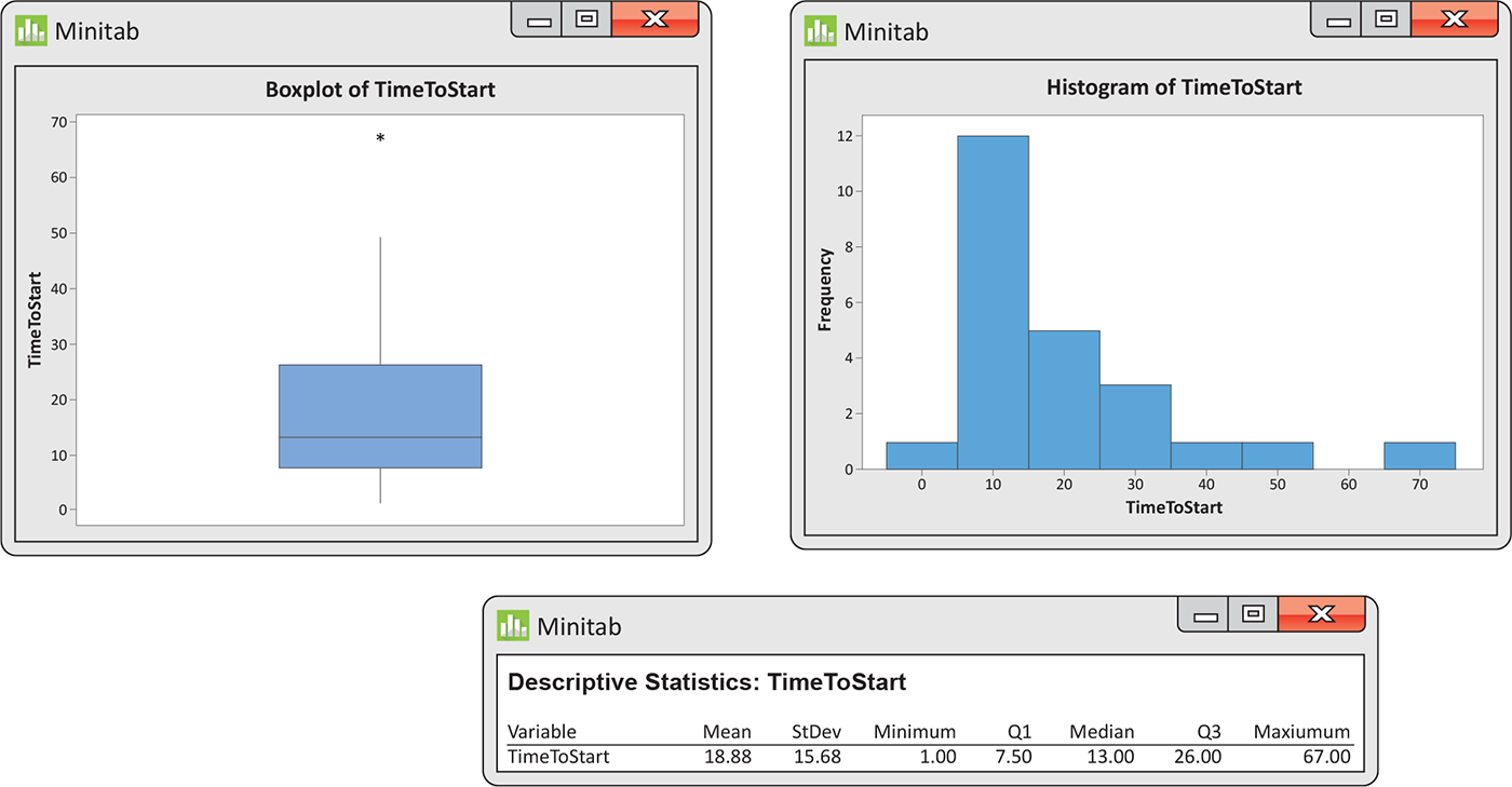
Figure 1.16 Graphical and numerical summaries from Minitab: boxplot, histogram, and numerical summaries for the time to start a business, Example 1.29.
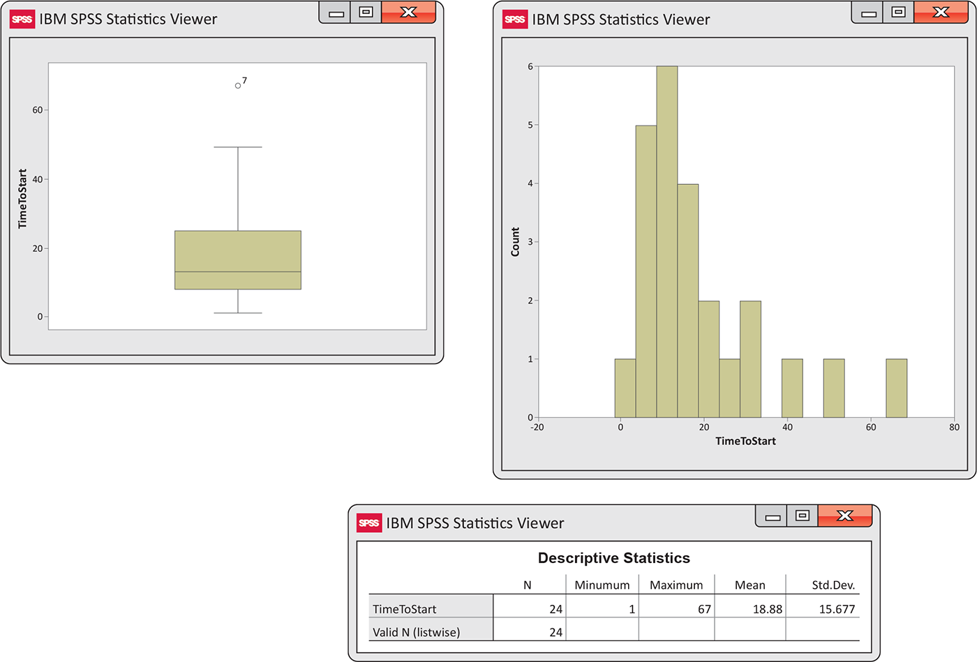
Figure 1.17 Graphical and numerical summaries from SPSS: boxplot, histogram, and numerical summaries for the time to start a business, Example 1.29.
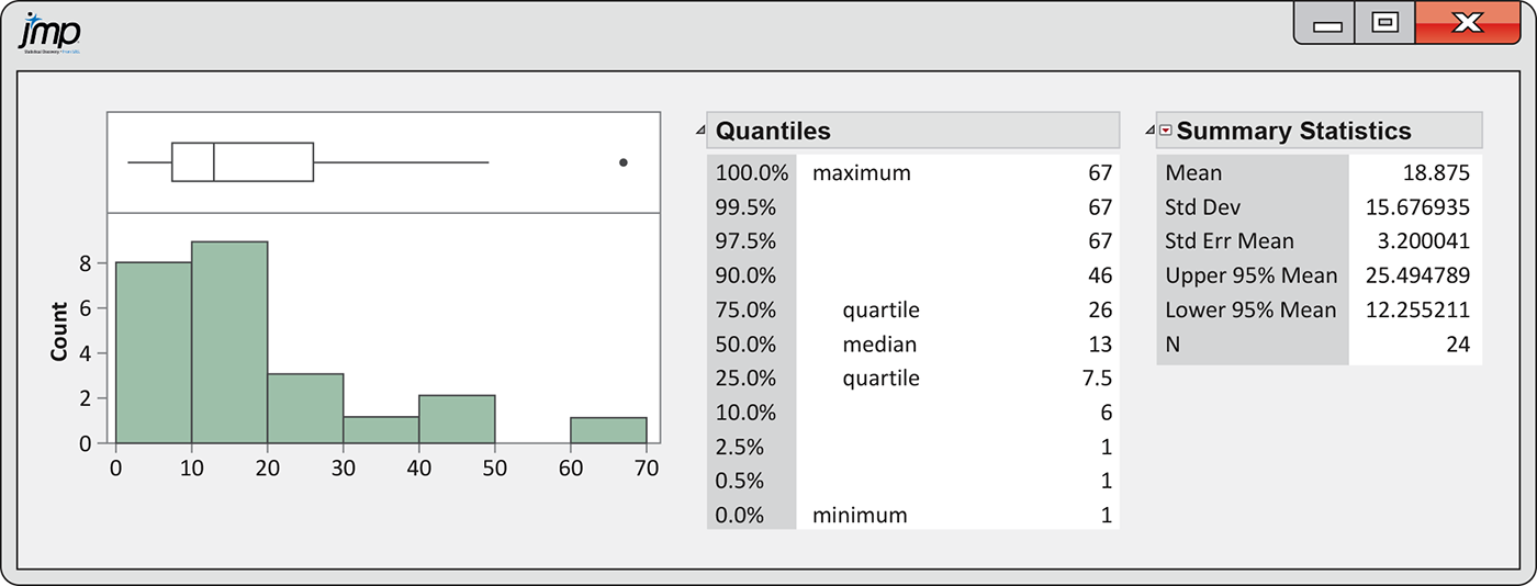
Figure 1.18 Graphical and numerical summaries from JMP for the time to start a business, Example 1.29.
Changing the unit of measurement
The same variable can be recorded in different units of measurement. Americans commonly record distances in miles and temperatures in degrees Fahrenheit, while the rest of the world measures distances in kilometers and temperatures in degrees Celsius. Fortunately, it is easy to convert numerical descriptions of a distribution from one unit of measurement to another. This is true because a change in the measurement unit is a linear transformation of the measurements.
Example 1.30 Change the units.
-
A temperature
Thus, the high of 95°F on a hot American summer day translates into 35°C. In this case,
This linear transformation changes both the unit size and the origin of the measurements. The origin in the Celsius scale (
-
If a distance
For example, a 10-kilometer race covers 6.2 miles. This transformation changes the units without changing the origin; a distance of 0 kilometers is the same as a distance of 0 miles.
Linear transformations do not change the shape of a
distribution.
If measurements on a variable
Although a linear transformation preserves the basic shape of a distribution, the center and spread will change. Because linear changes of measurement scale are common, we must be aware of their effect on numerical descriptive measures of center and spread. Fortunately, the changes follow a simple pattern.
Example 1.31 Use scores to find the points.
In an introductory statistics course, homework counts for 300 points out of a total of 1000 possible points for all course requirements. During the semester, there were 12 homework assignments, and each was given a grade on a scale of 0 to 100. The maximum total score for the 12 homework assignments is therefore 1200. To convert the homework scores to final grade points, we need to convert the scale of 0 to 1200 to a scale of 0 to 300. We do this by multiplying the homework scores by 300/1200. In other words, we divide the homework scores by 4. Here are the homework scores and the corresponding final grade points for five students:
| Student | 1 | 2 | 3 | 4 | 5 |
|---|---|---|---|---|---|
| Score | 1056 | 1080 | 900 | 1164 | 1020 |
| Points | 264 | 270 | 225 | 291 | 255 |
These two sets of numbers measure the same performance on homework for the course. Because we obtained the points by dividing the scores by 4, the mean of the points will be the mean of the scores divided by 4. Similarly, the standard deviation of points will be the standard deviation of the scores divided by 4.
Check-in
-
1.28 Calculate the points for a student. Use the setting of Example 1.31 to find the points for a student whose score is 960.
Here is a summary of the rules for linear transformations.
In Example 1.31, when we converted from score to points, we described the transformation as dividing by 4. The multiplication part of the summary of the effect of a linear transformation applies to this case because division by 4 is the same as multiplication by 0.25. Similarly, the second part of the summary applies to subtraction as well as addition because subtraction is simply the addition of a negative number.
The measures of spread IQR and
Section 1.3 SUMMARY
-
A numerical summary of a distribution should report its center and its spread or variability.
-
The mean
-
When you use the median to describe the center of a distribution, describe its spread by giving the quartiles. The first quartile
-
The interquartile range is the difference between the quartiles. It is the spread of the center half of the data. The
-
The five-number summary—consisting of the median, the quartiles, and the smallest and largest individual observations—provides a quick overall description of a distribution. The median describes the center, and the quartiles and extremes show the spread.
-
Boxplots based on the five-number summary are useful for comparing several distributions. The box spans the quartiles and shows the spread of the central half of the distribution. The median is marked within the box. Lines extend from the box to the extremes and show the full spread of the data. In a modified boxplot, points identified by the
-
The variance
-
A resistant measure of any aspect of a distribution is relatively unaffected by changes in the numerical value of a small proportion of the total number of observations, no matter how large these changes are. The median and quartiles are resistant, but the mean and the standard deviation are not.
-
The mean and standard deviation are good descriptions for symmetric distributions without outliers. They are most useful for the Normal distributions introduced in the next section. The five-number summary is a better exploratory description for skewed distributions.
-
Linear transformations have the form
-
Numerical measures of particular aspects of a distribution, such as center and spread, do not report the entire shape of most distributions. In some cases, particularly distributions with multiple peaks and gaps, these measures may not be very informative.
Section 1.3 EXERCISES
-
1.28 What’s wrong? Explain what is wrong with each of the following:
-
The mean is a resistant measure of the center of a distribution.
-
If you multiply a variable by 10, you do not change the value of the mean.
-
The five number summary includes the mean and the standard deviation.
-
-
1.29 Potassium from potatoes. Refer to Exercise 1.15 (page 22), where you examined the potassium absorption of a group of 27 adults who ate a controlled diet that included 40 mEq of potassium from potatoes for five days.

-
Compute the mean for these data.
-
Compute the median for these data.
-
Which measure do you prefer for describing the center of this distribution: the mean or the median? Explain your answer. (You may include a graphical summary as part of your explanation.)
-
-
1.30 Potassium from a supplement. Refer to Exercise 1.16 (page 22), where you examined the potassium absorption of a group of 29 adults who ate a controlled diet that included 40 mEq of potassium from a supplement for five days.

-
Compute the mean for these data.
-
Compute the median for these data.
-
Which measure do you prefer for describing the center of this distribution: the mean or the median? Explain your answer. (You may include a graphical summary as part of your explanation.)
-
-
1.31 Potassium from potatoes. Refer to Exercise 1.15 (page 22), where you examined the potassium absorption of a group of 27 adults who ate a controlled diet that included 40 mEq of potassium from potatoes for five days.
-
Compute the standard deviation for these data.
-
Compute the quartiles for these data.
-
Give the five-number summary and explain the meaning of each of the five numbers.
-
Which numerical summary do you prefer for describing this distribution: the mean, the standard deviation, or the five-number summary? Explain your answer. (You may include a graphical summary as part of your explanation.)
-
-
1.32 Potassium from a supplement. Refer to Exercise 1.16 (page 22), where you examined the potassium absorption of a group of 29 adults who ate a controlled diet that included 40 mEq of potassium from a supplement for five days.
-
Compute the standard deviation for these data.
-
Compute the quartiles for these data.
-
Give the five-number summary and explain the meaning of each of the five numbers.
-
Which numerical summary do you prefer for describing this distribution: the mean, the standard deviation, or the five-number summary? Explain your answer. (You may include a graphical summary as part of your explanation.)
-
-
1.33 Potassium from potatoes. Refer to Exercise 1.15 (page 22), where you examined the potassium absorption of a group of 27 adults who ate a controlled diet that included 40 mEq of potassium from potatoes for five days. In Exercise 1.15, you used a stemplot to examine the distribution of the potassium absorption.
-
Make a histogram and use it to describe the distribution of potassium absorption.
-
Make a boxplot and use it to describe the distribution of potassium absorption.
-
Compare the stemplot, the histogram, and the boxplot as graphical summaries of this distribution. Which do you prefer? Give reasons for your answer.
-
-
1.34 Potassium from a supplement. Refer to Exercise 1.16 (page 22), where you examined the potassium absorption of a group of 29 adults who ate a controlled diet that included 40 mEq of potassium from a supplement for five days. In Exercise 1.16, you used a stemplot to examine the distribution of the potassium absorption.
-
Make a histogram and use it to describe the distribution of potassium absorption.
-
Make a boxplot and use it to describe the distribution of potassium absorption.
-
Compare the stemplot, the histogram, and the boxplot as graphical summaries of this distribution. Which do you prefer? Give reasons for your answer.
-
-
1.35 Compare the potatoes with the supplement. Refer to Exercises 1.15 and 1.16 (page 22).

-
Use a back-to-back stemplot to display the data for the two sources of potassium. Compare the two distributions and write a short summary of your findings.
-
Use side-by-side boxplots to display the data for the two sources of potassium. Compare the two distributions and write a short summary of your findings.
-
Do you prefer stemplots or boxplots to compare these distributions? Give reasons for your answer.
-
-
1.36 Potassium sources. The data for potassium absorption in the previous exercise were expressed in milligrams (mg). Convert the data to grams (g) and answer the questions given in the previous exercise. There are 1000 mg in 1 g, so 3000 mg is the same as 3 g. In what ways are your answers here similar to the ones you gave in the previous exercise?
-
1.37 Gosset’s data on double stout sales. William Sealy Gosset worked at the Guinness Brewery in Dublin and made substantial contributions to the practice of statistics.22 In his work at the brewery, he collected and analyzed a great deal of data. Archives with Gosset’s handwritten tables, graphs, and notes have been preserved at the Guinness Storehouse in Dublin.23 In one study, Gosset examined the change in the double stout market before and after World War I (1914–1918). For various regions in England and Scotland, he calculated the ratio of sales in 1925, after the war, as a percent of sales in 1913, before the war. Here are the data:

Bristol 94 Glasgow 66 Cardiff 112 Liverpool 140 English Agents 78 London 428 English O 68 Manchester 190 English P 46 Newcastle-on-Tyne 118 English R 111 Scottish 24 -
Compute the mean for these data.
-
Compute the median for these data.
-
Which measure do you prefer for describing the center of this distribution? Explain your answer. (You may include a graphical summary as part of your explanation.)
-
-
1.38 Measures of spread for the double stout data. Refer to the previous exercise.
-
Compute the standard deviation for these data.
-
Compute the quartiles for these data.
-
Which measure do you prefer for describing the spread of this distribution? Explain your answer. (You may include a graphical summary as part of your explanation.)
-
-
1.39 Are there outliers in the double stout data? Refer to the previous two exercises.
-
Find the IQR for these data.
-
Use the
-
Make a boxplot for these data and describe the distribution using only the information in the boxplot.
-
Make a modified boxplot for these data and describe the distribution using only the information in the boxplot.
-
Make a stemplot for these data.
-
Compare the boxplot, the modified boxplot, and the stemplot. Evaluate the advantages and disadvantages of each graphical summary for describing the distribution of the double stout data.
-
-
1.40 Smolts. Smolts are young salmon at a stage when their skin becomes covered with silvery scales, and they start to migrate from freshwater to the sea. The reflectance of a light shined on a smolt’s skin is a measure of the smolt’s readiness for the migration. Here are the reflectances, in percents, for a sample of 50 smolts:24

57.6 54.8 63.4 57.0 54.7 42.3 63.6 55.5 33.5 63.3 58.3 42.1 56.1 47.8 56.1 55.9 38.8 49.7 42.3 45.6 69.0 50.4 53.0 38.3 60.4 49.3 42.8 44.5 46.4 44.3 58.9 42.1 47.6 47.9 69.2 46.6 68.1 42.8 45.6 47.3 59.6 37.8 53.9 43.2 51.4 64.5 43.8 42.7 50.9 43.8 -
Find the mean reflectance for these smolts.
-
Find the median reflectance for these smolts.
-
Do you prefer the mean or the median as a measure of center for these data? Give reasons for your preference.
-
-
1.41 Measures of spread for smolts. Refer to the previous exercise.
-
Find the standard deviation of the reflectance for these smolts.
-
Find the quartiles of the reflectance for these smolts.
-
Do you prefer the standard deviation or the quartiles as a measure of spread for these data? Give reasons for your preference.
-
-
1.42 Are there outliers in the smolt data? Refer to the previous two exercises.
-
Find the IQR for the smolt data.
-
Use the
-
Make a boxplot for the smolt data and describe the distribution using only the information in the boxplot.
-
Make a modified boxplot for these data and describe the distribution using only the information in the boxplot.
-
Make a stemplot for these data.
-
Compare the boxplot, the modified boxplot, and the stemplot. Evaluate the advantages and disadvantages of each graphical summary for describing the distribution of the smolt reflectance data.
-
-
1.43 Potatoes. A quality product is one that is consistent and has very little variability in its characteristics. Controlling variability can be more difficult with agricultural products than with products that are manufactured. The following table gives the weights, in ounces, of the 25 potatoes sold in a 10-pound bag:

7.8 7.9 8.2 7.3 6.7 7.9 7.9 7.9 7.6 7.8 7.0 4.7 7.6 6.3 4.7 4.7 4.7 6.3 6.0 5.3 4.3 7.9 5.2 6.0 3.7 -
Summarize the data graphically and numerically. Give reasons for the methods you chose to use in your summaries.
-
Do you think that your numerical summaries do an effective job of describing these data? Why or why not?
-
There appear to be two distinct clusters of weights for these potatoes. Divide the sample into two subsamples based on the clustering. Give the mean and standard deviation for each subsample. Do you think that this way of summarizing these data is better than a numerical summary that uses all the data as a single sample? Give a reason for your answer.
-
-
1.44 The alcohol content of beer. Brewing beer involves a variety of steps that can affect the alcohol content. A website gives the percent alcohol for 160 domestic brands of beer.25 Use graphical and numerical summaries of your choice to describe the data. Give reasons for your choice.

-
1.45 Outliers for alcohol content of beer. Refer to the previous exercise.
-
Calculate the mean with and without the outliers. Do the same for the median. Explain how these values change when the outliers are excluded.
-
Calculate the standard deviation with and without the outliers. Do the same for the quartiles. Explain how these values change when the outliers are excluded.
-
Write a short paragraph summarizing what you have learned in this exercise.
-
-
1.46 Calories in beer. Refer to the previous two exercises. The data set also lists calories per 12 ounces of beverage.
-
Analyze the data and summarize the distribution of calories for these 160 brands of beer.
-
Are there any outliers? If yes, list them by name. How do these outliers compare with those you identified when analyzing the alcohol content?
-
-
1.47 Median versus mean for net worth. A report on the assets of American households says that the median net worth of U.S. families is $97,300. The mean net worth of these families is $692,100.26 What explains the difference between these two measures of center?
-
1.48 Create a data set. Create a data set with five observations for which the median would change by a large amount if the largest observation were deleted.
-
1.49 Mean versus median. A small accounting firm pays each of its six clerks $40,000, four junior accountants $46,000 each, and the firm’s owner $700,000. What is the mean salary paid at this firm? How many of the employees earn less than the mean? What is the median salary?
-
1.50 Be careful about how you treat the zeros. In computing the median income of any group, some federal agencies omit all members of the group who had no income. Give an example to show that the reported median income of a group can go down even though the group becomes economically better off. Is this also true of the mean income?
-
1.51 How does the median change? The firm in Exercise 1.49 gives no raises to the clerks and junior accountants, while the owner’s take increases to $950,000. How does this change affect the mean? How does it affect the median?
-
1.52 Metabolic rates. Calculate the mean and standard deviation of the metabolic rates in Example 1.28 (page 36), showing each step in detail. First find the mean

-
 1.53 Mean and median for two observations.
The Mean and Median applet allows you to place
observations on a line and see their mean and median visually.
Place two observations on the line by clicking below it. Why
does only one arrow appear?
1.53 Mean and median for two observations.
The Mean and Median applet allows you to place
observations on a line and see their mean and median visually.
Place two observations on the line by clicking below it. Why
does only one arrow appear?
-
1.54 Mean and median for six observations. In
the Mean and Median applet, place six observations on the
line by clicking below it, five close together near the center
of the line, and one somewhat to the right of these five.
-
Pull the single rightmost observation out to the right. (Place the cursor on the point, hold down a mouse button, and drag the point.) How does the mean behave? How does the median behave? Explain briefly why each measure acts as it does.
-
Now drag the rightmost point to the left as far as you can. What happens to the mean? What happens to the median as you drag this point past the other five?
-
-
1.55 Imputation. Various problems with data collection can cause some observations to be missing. Suppose a data set has 20 cases. Here are the values of the variable
18 9 12 15 20 23 9 12 16 21 The values for the other 10 cases are missing. One way to deal with missing data is called imputation. The basic idea is that missing values are replaced, or imputed, with values that are based on an analysis of the data that are not missing. For a data set with a single variable, the usual choice of a value for imputation is the mean of the values that are not missing. The mean for this data set is 16.

-
Verify that the mean is 16 and find the standard deviation for the 10 cases for which
-
Create a new data set with 20 cases by setting the values for the 10 missing cases to 16. Compute the mean and standard deviation for this data set.
-
Summarize what you have learned about the possible effects of this type of imputation on the mean and the standard deviation.
-
-
1.56 Longleaf pine trees. The Wade Tract in Thomas County, Georgia, is an old-growth forest of longleaf pine trees (Pinus palustris) that has survived in a relatively undisturbed state since before the settlement of the area by Europeans. A study collected data on 584 of these trees.27 One of the variables measured was the diameter at breast height (DBH). This is the diameter of the tree at 4.5 feet, and the units are centimeters (cm). Only trees with DBH greater than 1.5 cm were sampled. Here are the diameters of a random sample of 40 of these trees:

10.5 13.3 26.0 18.3 52.2 9.2 26.1 17.6 40.5 31.8 47.2 11.4 2.7 69.3 44.4 16.9 35.7 5.4 44.2 2.2 4.3 7.8 38.1 2.2 11.4 51.5 4.9 39.7 32.6 51.8 43.6 2.3 44.6 31.5 40.3 22.3 43.3 37.5 29.1 27.9 -
Find the five-number summary for these data.
-
Make a boxplot.
-
Make a histogram.
-
Write a short summary of the major features of this distribution. Do you prefer the boxplot or the histogram for these data?
-
-
1.57 Weight gain. A study of diet and weight gain deliberately overfed 15 volunteers for eight weeks. The mean increase in fat was
-
1.58 Changing units from inches to centimeters. Changing the unit of length from inches to centimeters multiplies each length by 2.54 because there are 2.54 centimeters in an inch. This change of units multiplies our usual measures of spread by 2.54. This is true of IQR and the standard deviation. What happens to the variance when we change units in this way?
-
 1.59 A different type of mean.
The trimmed mean is a measure of center that is more
resistant than the mean but uses more of the available
information than the median. To compute the 10% trimmed mean,
discard the highest 10% and the lowest 10% of the observations
and compute the mean of the remaining 80%. Trimming eliminates
the effect of a small number of outliers. Compute the 10%
trimmed mean of the beer alcohol data in
Exercise 1.44 (page 45). Then compute the 20% trimmed mean. Compare the values of
these measures with the median and the ordinary untrimmed mean.
1.59 A different type of mean.
The trimmed mean is a measure of center that is more
resistant than the mean but uses more of the available
information than the median. To compute the 10% trimmed mean,
discard the highest 10% and the lowest 10% of the observations
and compute the mean of the remaining 80%. Trimming eliminates
the effect of a small number of outliers. Compute the 10%
trimmed mean of the beer alcohol data in
Exercise 1.44 (page 45). Then compute the 20% trimmed mean. Compare the values of
these measures with the median and the ordinary untrimmed mean.
-
1.60 Changing units from centimeters to inches. Refer to Exercise 1.56. Change the measurements from centimeters to inches by multiplying each value by 0.39. Answer the questions from that exercise and explain the effect of the transformation on these data.