1.4 Density Curves and Normal Distributions
We now have a kit of graphical and numerical tools for describing distributions. What is more, we have a clear strategy for exploring data on a single quantitative variable:
- Always plot your data: make a graph, usually a stemplot or a histogram.
- Look for the overall pattern and for striking deviations such as outliers.
- Calculate an appropriate numerical summary to briefly describe center and spread.
Technology has expanded the set of graphs that we can choose for Step 1. It is possible, though painful, to make histograms by hand. Using software, clever algorithms can describe a distribution in a way that is not feasible by hand, by fitting a smooth curve to the data in addition to or instead of a histogram. The curves used are called density curves. Before we examine density curves in detail, here is an example of what software can do.
Example 1.32 Density curve for times to start a business.
![]()
Figure 1.19 illustrates the use of a density curve along with a histogram to describe distributions. It shows the distribution of the times to start a business for 186 countries (see Example 1.19, page 26). The outlier, Venezuela, described in Check-in question 1.16 (page 27), has been deleted from the data set. The distribution is highly skewed to the right. Most of the data are in the first several classes, with 50 or fewer days to start a business, but there are a few countries with very large start times.
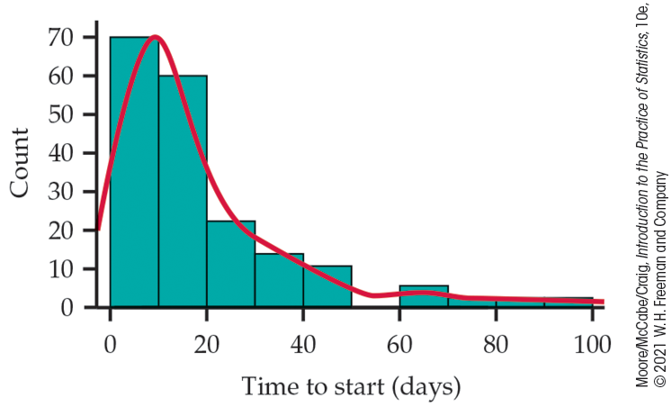
Figure 1.19 The distribution of 186 times to start a business, Example 1.32. Venezuela, the outlier, has been eliminated from this plot. The distribution is pictured with both a histogram and a density curve. This distribution has a single mode with a long tail.
A smooth density curve is an idealization that gives the overall pattern of the data but ignores minor irregularities. We first discuss density curves in general and then focus on a special class of density curves, the bell-shaped Normal curves.
Density curves
One way to think of a density curve is as a smooth approximation to the irregular bars of a histogram. Figure 1.20 shows a histogram of the scores of all 947 seventh-grade students in Gary, Indiana, on the vocabulary part of the Iowa Test of Basic Skills. Scores of many students on this national test have a very regular distribution. The histogram is symmetric, and both tails fall off quite smoothly from a single center peak. There are no large gaps or obvious outliers. The curve drawn through the tops of the histogram bars in Figure 1.20 is a good description of the overall pattern of the data.
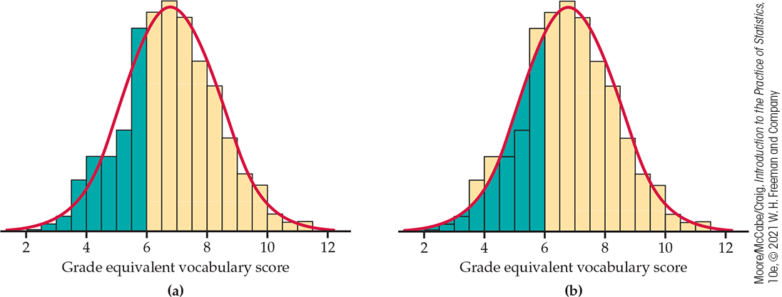
Figure 1.20 (a) The distribution of Iowa Test vocabulary scores for Gary, Indiana, seventh-graders, Example 1.33. The shaded bars in the histogram represent scores less than or equal to 6.0. (b) The shaded area under the Normal density curve also represents scores less than or equal to 6.0. This area is 0.293, close to the true 0.303 for the actual data.
Example 1.33 Vocabulary scores.
In a histogram, the heights of the bars represent either counts or
proportions of the observations. In
Figure 1.20(a), we shaded
the bars that represent students with vocabulary scores 6.0 or
lower. There are 287 such students, who make up the proportion
In Figure 1.20(b), we
shaded the area under the curve to the left of 6.0. If we adjust the
scale so that the total area under the curve is exactly 1, areas
under the curve will then represent proportions of the observations.
That is,
The density curve in Figure 1.20 is a Normal curve. Density curves, like distributions, come in many shapes. Figure 1.21 shows two density curves: a symmetric Normal density curve and a right-skewed curve.
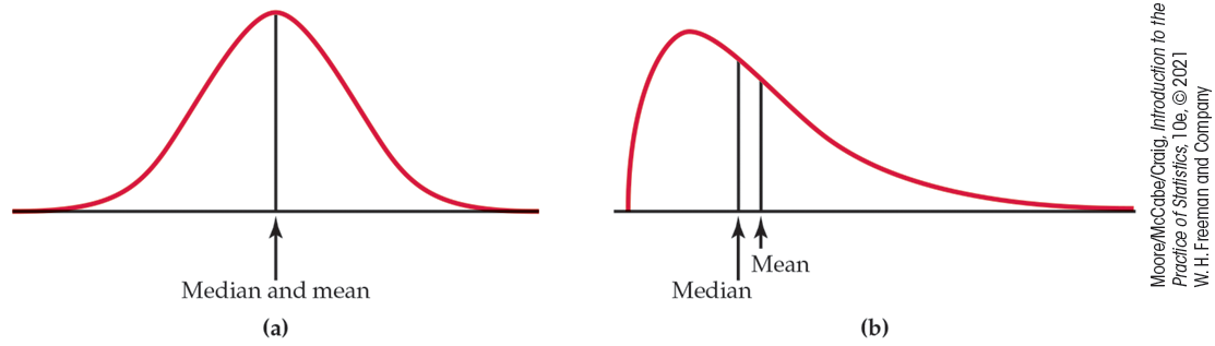
Figure 1.21 (a) A symmetric Normal density curve with its mean and median marked. (b) A right-skewed density curve with its mean and median marked.
We will discuss Normal density curves in detail in this section because of the important role they play in statistics. There are, however, many applications where the use of other families of density curves are essential.
A density curve of an appropriate shape is often an adequate description of the overall pattern of a distribution. Outliers, which are deviations from the overall pattern, are not described by the curve.
Measuring center and spread for density curves
Our measures of center and spread apply to density curves as well as to actual sets of observations, but only some of these measures are easily seen from the curve. A mode of a distribution described by a density curve is a peak point of the curve, the location where the curve is highest. Because areas under a density curve represent proportions of the observations, the median is the point with half the total area on each side. You can roughly locate the quartiles by dividing the area under the curve into quarters as accurately as possible by eye. The IQR is the distance between the first and third quartiles. There are mathematical ways of calculating areas under curves. These allow us to locate the median and quartiles exactly on any density curve.
What about the mean and standard deviation? The mean of a set of observations is their arithmetic average. If we think of the observations as weights strung out along a thin rod, the mean is the point at which the rod would balance. This fact is also true of density curves. The mean is the point at which the curve would balance if it were made out of solid material. Figure 1.22 illustrates this interpretation of the mean.
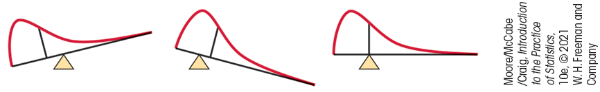
Figure 1.22 The mean of a density curve is the point at which it would balance.
A symmetric curve, such as the Normal curve in Figure 1.21(a), balances at its center of symmetry. Half the area under a symmetric curve lies on either side of its center, so this is also the median.
For a right-skewed curve, such as those shown in Figures 1.21(b) and 1.22, the small area in the long right tail tips the curve more than the same area near the center. The mean (the balance point), therefore, lies to the right of the median. It is hard to locate the balance point by eye on a skewed curve. There are mathematical ways of calculating the mean for any density curve, so we are able to mark the mean as well as the median in Figure 1.21(b). The standard deviation can also be calculated mathematically, but it can’t be located by eye on most density curves.
A density curve is an idealized description of a distribution of data.
For example, the density curve in
Figure 1.20 (page 47) is exactly symmetric, but the histogram of vocabulary scores is
only approximately symmetric. We therefore need to distinguish between
the mean and standard deviation of the density curve and the numbers
Normal distributions
One particularly important class of density curves has already appeared in Figures 1.20 and 1.21(a). These density curves are symmetric, unimodal, and bell-shaped. They are called Normal curves, and they describe Normal distributions. All Normal distributions have the same overall shape.
The exact density curve for a particular Normal distribution is
specified by giving the distribution’s mean
The standard deviation
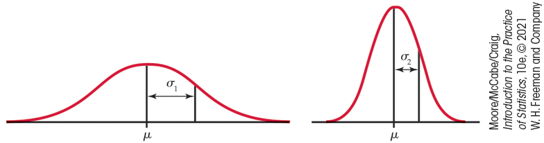
Figure 1.23 Two Normal
curves, both showing the same mean
The standard deviation
The points at which this change of curvature takes place are located
at distance
![]() Remember that
Remember that
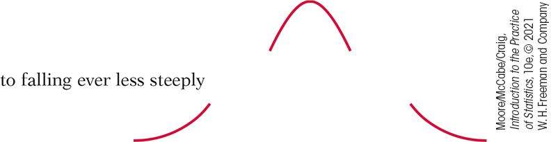
There are other symmetric bell-shaped density curves that are not
Normal. The Normal density curves are specified by a particular
equation. The height of the density curve at any point
We will not make direct use of this fact, although it is the basis of
mathematical work with Normal distributions. Notice that the equation
of the curve is completely determined by the mean
Why are the Normal distributions important in statistics? Here are three reasons:
-
Normal distributions are good descriptions for some distributions of real data. Distributions that are often close to Normal include scores on tests taken by many people (such as the Iowa Test of Figure 1.20, page 47), repeated careful measurements of the same quantity, and characteristics of biological populations (such as lengths of baby pythons and yields of corn).
-
Normal distributions are good approximations to the results of many kinds of chance outcomes, such as tossing a coin many times.
-
Many statistical inference procedures based on Normal distributions work well for other roughly symmetric distributions.
![]() However,
even though many sets of data follow a Normal distribution, many do
not.
Most income distributions, for example, are skewed to the right and so
are not Normal. Non-Normal data, like nonnormal people, not only are
common but are also sometimes more interesting than their Normal
counterparts.
However,
even though many sets of data follow a Normal distribution, many do
not.
Most income distributions, for example, are skewed to the right and so
are not Normal. Non-Normal data, like nonnormal people, not only are
common but are also sometimes more interesting than their Normal
counterparts.
The 68–95–99.7 rule
Although there are many Normal curves, they all have common properties. Here is one of the most important.
Figure 1.24 illustrates the 68–95–99.7 rule. By remembering these three numbers, you can think about Normal distributions without constantly making detailed calculations.
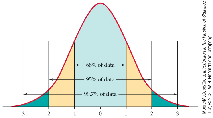
Figure 1.24 The 68–95–99.7 rule for Normal distributions.
Example 1.34 Heights of young women.
The distribution of heights of young women aged 18 to 24 is
approximately Normal with mean
Two standard deviations equals five inches for this distribution.
The 95 part of the 68–95–99.7 rule says that the middle 95% of young
women are between
The other 5% of young women have heights outside the range from 59.5 to 69.5 inches. Because the Normal distributions are symmetric, half of these women are on the tall side. So the tallest 2.5% of young women are taller than 69.5 inches.
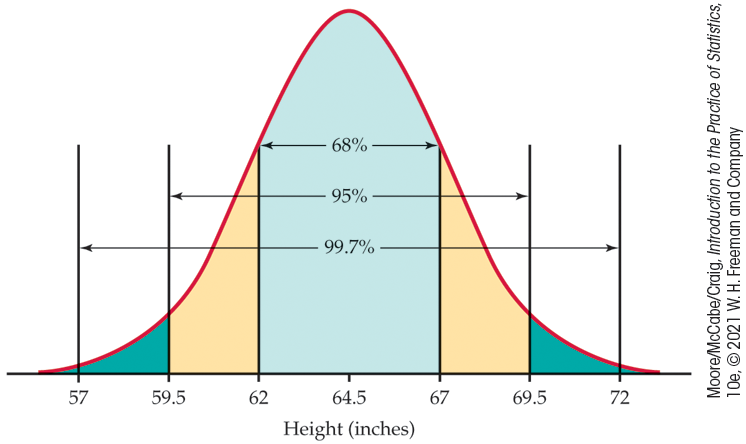
Figure 1.25 The 68–95–99.7 rule applied to the heights of young women, Example 1.34.
Because we will mention Normal distributions often, a short notation
is helpful. We abbreviate the Normal distribution with mean
Check-in
-
1.29 Test scores. Many states assess the skills of their students in various grades. One program that is available for this purpose is the National Assessment of Educational Progress (NAEP).28 One of the tests provided by the NAEP assesses the mathematics skills of eighth-grade students. In a recent year, the national mean score was 282, and the standard deviation was 40. Assuming that these scores are approximately Normally distributed,
-
1.30 Use the 68–95–99.7 rule. Refer to the previous Check-in question. Use the 68–95–99.7 rule to give a range of scores that includes 99.7% of these students.
Standardizing observations
As the 68–95–99.7 rule suggests, all Normal distributions share many
properties. In fact, all Normal distributions are the same if we
measure in units of size
A
To compare scores based on different measures,
Example 1.35 Find some z-scores.
The heights of young women are approximately Normal with
A woman’s standardized height is the number of standard deviations
by which her height differs from the mean height of all young women.
A woman 68 inches tall, for example, has
or a height that is 1.4 standard deviations above the mean.
Similarly, a woman 5 feet (60 inches) tall has
or a height that is 1.8 standard deviations less than the mean.
Check-in
-
1.31 Find the z-score. Consider the NAEP scores (see Check-in question 1.29, page 52), which we assume are approximately Normal,
-
1.32 Find another z-score. Consider the NAEP scores, which we assume are approximately Normal,
We need a way to write variables, such as “height” in
Example 1.34, that
follow a theoretical distribution such as a Normal distribution. We
use capital letters near the end of the alphabet for such variables.
If
We often standardize observations from symmetric distributions to
express them in a common scale. We might, for example, compare the
heights of two children of different ages by calculating their
Standardizing is a linear transformation that transforms the data into
the standard scale of
If the variable we standardize has a Normal distribution, standardizing does more than give a common scale. It makes all Normal distributions into a single distribution, and this distribution is still Normal. Standardizing a variable that has any Normal distribution produces a new variable that has the standard Normal distribution.
Normal distribution calculations
Areas under a Normal curve represent proportions of observations from that Normal distribution. There is no formula for areas under a Normal curve. Calculations use either software that calculates areas or a table of areas. The table and most software calculate one kind of area: cumulative proportion, which is the proportion of observations in a distribution that lie at or below a given value. When the distribution is given by a density curve, the cumulative proportion is the area under the curve to the left of a given value. Figure 1.26 shows the idea more clearly than words do.
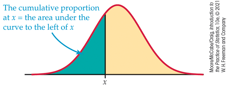
Figure 1.26 The
cumulative proportion for a value
The key to calculating Normal proportions is to match the area you want with areas that represent cumulative proportions. Then get areas for cumulative proportions either from software or (with an extra step) from a table. The following examples show the method in pictures.
Example 1.36 The NCAA standard for SAT scores.
The National Collegiate Athletic Association (NCAA) requires Division I athletes to get a combined score of at least 820 on the SAT Mathematics and Verbal tests to compete in their first college year.29 (Higher scores are required for students with poor high school grades.) The scores of the 1.4 million students who took the SATs were approximately Normal with mean 1026 and standard deviation 209. What proportion of all students had SAT scores of at least 820?
Here is the calculation in pictures: the proportion of scores above 820 is the area under the curve to the right of 820. That’s the total area under the curve (which is always 1) minus the cumulative proportion up to 820. Note that we have used software for these calculations.
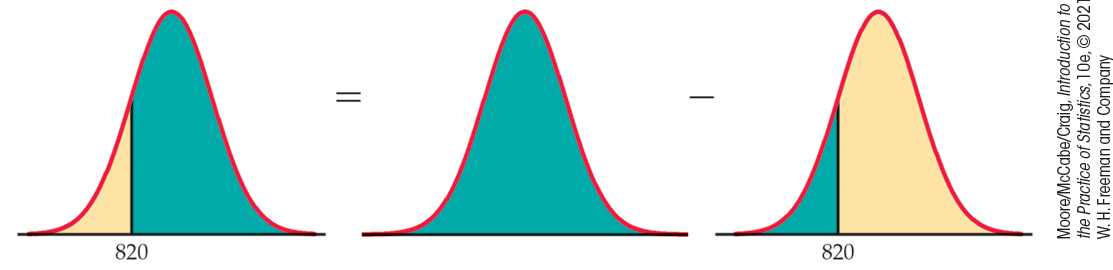
Thus, the proportion of all SAT test-takers who would be NCAA qualifiers is 0.8378, or about 84%.
There is no area under a smooth curve that is exactly over the
point 820. Consequently, the area to the right of 820 (the proportion
of scores
Example 1.37 Partial qualifiers.
The NCAA considers a student to be a “partial qualifier”—eligible to practice and receive an athletic scholarship, but not compete—if the combined SAT score is at least 720.30 What proportion of all students who take the SAT would be partial qualifiers? That is, what proportion have scores between 720 and 820? Here are the pictures:
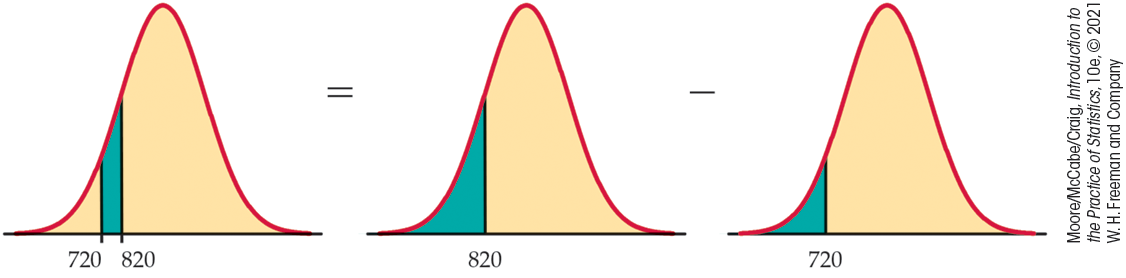
About 9% of all students who take the SAT have scores between 720 and 820.
How do we find the numerical values of the areas in Examples 1.36 and 1.37? If you use software, just plug in mean 1026 and standard deviation 209. Then ask for the cumulative proportions for 820 and for 720. (Your software will probably refer to these as “cumulative probabilities.” We will learn in Chapter 4 why the language of probability fits.) Sketches of the areas that you want similar to the ones in Examples 1.36 and 1.37 are very helpful in making sure that you are doing the correct calculations.
![]() You can use the Normal Curve applet on the text website to find
Normal proportions. The applet is more flexible than most software—it
will find any Normal proportion, not just cumulative proportions. The
applet is an excellent way to understand Normal curves. But, because
of the limitations of web browsers, the applet is not as accurate as
statistical software.
You can use the Normal Curve applet on the text website to find
Normal proportions. The applet is more flexible than most software—it
will find any Normal proportion, not just cumulative proportions. The
applet is an excellent way to understand Normal curves. But, because
of the limitations of web browsers, the applet is not as accurate as
statistical software.
If you are not using software, you can find cumulative proportions for Normal curves from a table. That requires an extra step, as we now explain.
Using the standard Normal table
The extra step in finding cumulative proportions from a table is that
we must first standardize to express the problem in the standard scale
of
Example 1.38 Find the proportion from z.
What proportion of observations on a standard Normal variable
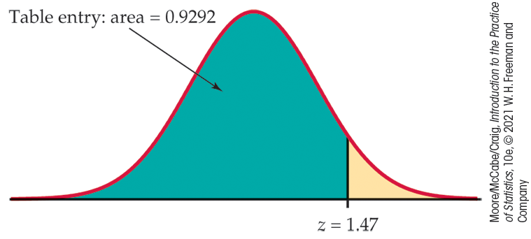
Figure 1.27 The area
under a standard Normal curve to the left of the point
Now that you see how Table A works, let’s redo the NCAA Examples 1.36 and 1.37 using the table.
Example 1.39 Find the proportion from x.
What proportion of college-bound students who take the SAT have
scores of at least 820? The picture that leads to the answer is
exactly the same as in
Example 1.36. The
extra step is that we first standardize to read cumulative
proportions from
Table A. If
-
Standardize. Subtract the mean, then divide by the standard deviation, to transform the problem about
-
Use the table. Look at the pictures in Example 1.36. From Table A, we see that the proportion of observations less than
The area from the table in
Example 1.39 (0.8389) is
slightly less accurate than the area from software in
Example 1.36 (0.8378)
because we must round
Example 1.40 Eligibility for aid and practice.
What proportion of all students who take the SAT would be eligible
to receive athletic scholarships and to practice with the team but
would not be eligible to compete in the eyes of the NCAA? That is,
what proportion of students have SAT scores between 720 and 820?
First, sketch the areas, exactly as in
Example 1.37. We again
use
-
Standardize.
-
Use the table.
As in Example 1.37, about 9% of students would be eligible to receive athletic scholarships and to practice with the team.
Sometimes we encounter a value of
Check-in
-
1.33 Find the proportion. Consider the NAEP scores, which are approximately Normal,
-
1.34 Find another proportion. Consider the NAEP scores, which are approximately Normal,
Inverse Normal calculations
Examples 1.36 to 1.40 illustrate the use of Normal distributions to find the proportion of observations in a given event, such as “SAT score between 720 and 820.” We may instead want to find the observed value corresponding to a given proportion.
Statistical software will do this directly. Without software, use
Table A
backward, finding the desired proportion in the body of the table and
then reading the corresponding
Example 1.41 How high for the top 10%?
Scores for college-bound students on the SAT Verbal test in recent
years follow approximately the
Again, the key to the problem is to draw a picture.
Figure 1.28
shows that we want the score
Statistical software has a function that will give you the
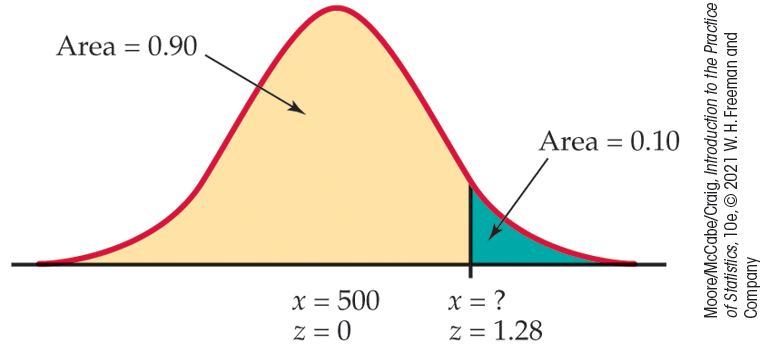
Figure 1.28 Locating the point on a Normal curve with area 0.10 to its right, Example 1.41.
Without software, first find the standard score
-
Use the table. Look in the body of Table A for the entry closest to 0.9. It is 0.8997. This is the entry corresponding to
-
Unstandardize to transform the solution from
Solving this equation for
This equation should make sense: it finds the
Check-in
-
1.35 What score is needed to be in the top 20%? Consider the NAEP scores, which are approximately Normal,
-
1.36 Find the score that 75% of students will exceed. Consider the NAEP scores, which are approximately Normal,
Normal quantile plots
The Normal distributions provide good descriptions of some distributions of real data, such as the Iowa Test vocabulary scores. The distributions of some other common variables are usually skewed and therefore distinctly non-Normal. Examples include economic variables such as personal income and gross sales of business firms, the survival times of cancer patients after treatment, and the service lifetime of mechanical or electronic components. While experience can suggest whether or not a Normal distribution is plausible in a particular case, it is risky to assume that a distribution is Normal without actually inspecting the data.
A histogram or stemplot can reveal distinctly non-Normal features of a distribution, such as outliers, pronounced skewness, or gaps and clusters. If the stemplot or histogram appears roughly symmetric and unimodal, however, we need a more sensitive way to judge the adequacy of a Normal model. The most useful tool for assessing Normality is another graph, the Normal quantile plot.
Here is the basic idea of a Normal quantile plot. The graphs produced by software use more sophisticated versions of this idea. It is not practical to make Normal quantile plots by hand.
-
Arrange the observed data values from smallest to largest. Record what percentile of the data each value occupies. For example, the smallest observation in a set of 20 is at the 5% point, the second smallest is at the 10% point, and so on.
-
Do Normal distribution calculations to find the values of
-
Plot each data point
Any Normal distribution produces a straight line on the plot because standardizing turns any Normal distribution into a standard Normal distribution. Standardizing is a linear transformation that can change the slope and intercept of the line in our plot but cannot turn a line into a curved pattern.
Figures 1.29 and
1.30 are Normal quantile
plots for data we have met earlier. The data
Example 1.42 IQ scores are approximately Normal.
![]()
Figure 1.29 is a Normal quantile plot of the 60 fifth-grade IQ scores from Table 1.1 (page 15). The points lie very close to the straight line drawn on the plot. We conclude that the distribution of IQ data is approximately Normal.
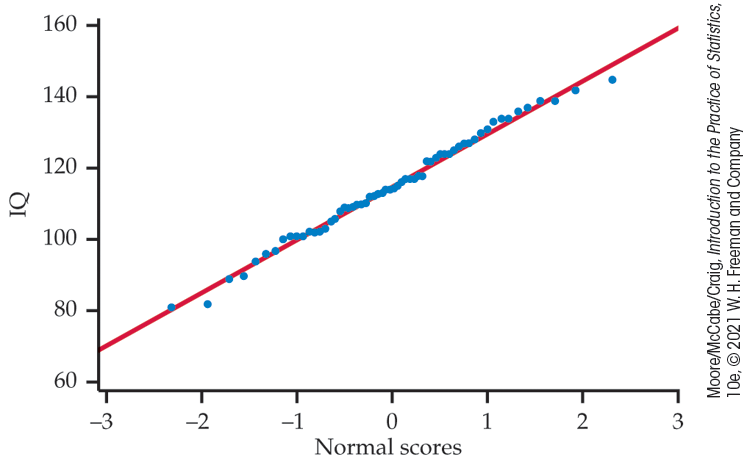
Figure 1.29 Normal quantile plot of IQ scores, Example 1.42. This distribution is approximately Normal.
Example 1.43 Times to start a business are skewed.
![]()
Figure 1.30 is a Normal quantile plot of the data on times to start a business from Example 1.19. The line drawn on the plot shows clearly that the plot of the data is curved. We conclude that these data are not Normally distributed. The shape of the curve is what we typically see with a distribution that is strongly skewed to the right.
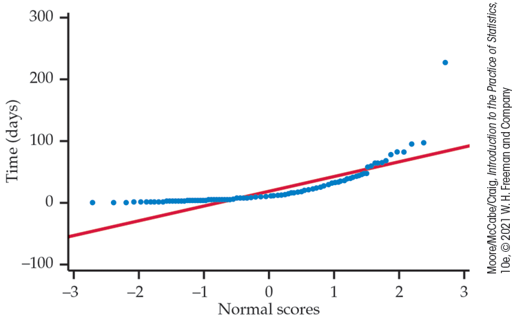
Figure 1.30 Normal quantile plot for the length of time required to start a business, Exercise 1.43. This distribution is highly skewed.
Real data often show some departure from the theoretical Normal
model.
![]() When you examine a Normal quantile plot, look for shapes that show
clear departures from Normality. Don’t overreact to minor wiggles in
the plot.
When we discuss statistical methods that are based on the Normal
model, we are interested in whether or not the data are sufficiently
Normal for these procedures to work properly We are not concerned
about minor deviations from Normality. Many common methods work well
as long as the data are approximately Normal and outliers are not
present.
When you examine a Normal quantile plot, look for shapes that show
clear departures from Normality. Don’t overreact to minor wiggles in
the plot.
When we discuss statistical methods that are based on the Normal
model, we are interested in whether or not the data are sufficiently
Normal for these procedures to work properly We are not concerned
about minor deviations from Normality. Many common methods work well
as long as the data are approximately Normal and outliers are not
present.
Example 1.44 Density estimation for IQ scores.
![]()
In Example 1.42 we observed that the points in the Normal quantile plot for the IQ data were very close to a straight line. This suggests that a Normal distribution is a good fit for these data. Figure 1.31 provides another way to look at this issue. Here we see the histogram with a density estimate, the red curve, along with the best-fitting Normal density curve, the green curve. Because the two curves are approximately the same, we are confident in any further analysis of these data based on the assumption that the data are approximately Normal.
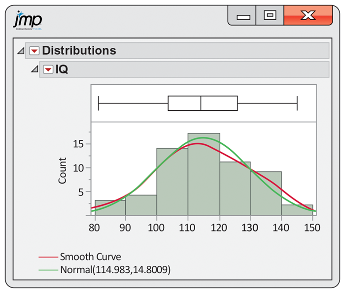
Figure 1.31 Histogram of IQ scores, with a density estimate and a Normal curve, Example 1.44. The IQ scores are approximately Normal.
![]()
Here is another example where we see a different picture.
Example 1.45 Density estimation for times to start a business.
![]()
In Example 1.43, we examined the Normal quantile plot for the time to start a business data. Figure 1.32 shows the histogram for these data along with a density estimate and the best-fitting Normal distribution. The two density curves are very different, and we conclude that a Normal distribution does not give a good fit for these data. Not only are the data strongly skewed, but there is also a clear outlier. We should be very cautious about using a statistical analysis based on an assumption that the data are approximately Normal in this case.
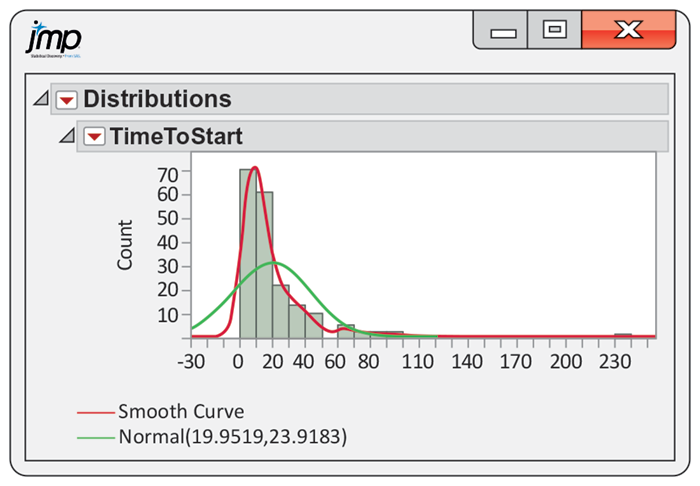
Figure 1.32 Histogram of the length of time required to start a business, with a density estimate and a Normal curve, Example 1.45. The Normal distribution is not a good fit for these data.
![]()
Section 1.4 SUMMARY
-
We can describe the overall pattern of a distribution by a density curve. A density curve has total area 1 underneath it. An area under a density curve gives the proportion of observations that fall in a range of values.
-
A density curve is an idealized description of the overall pattern of a distribution that smooths out the irregularities in the actual data. We write the mean of a density curve as
-
The mean
-
The mean and median are equal for symmetric density curves, but the mean of a skewed curve is located farther toward the long tail than is the median.
-
The Normal distributions are described by a special family of bell-shaped, symmetric, unimodal density curves. The mean
-
To standardize any observation
-
All Normal distributions are the same when measurements are transformed to the standardized scale. In particular, all Normal distributions satisfy the 68–95–99.7 rule, which describes what percent of observations lie within one, two, and three standard deviations of the mean.
-
If
-
The adequacy of a Normal model for describing a distribution of data is best assessed by a Normal quantile plot, which is available in most statistical software packages. A pattern on such a plot that deviates substantially from a straight line indicates that the data are not Normal.
Section 1.4 EXERCISES
-
1.61 What’s wrong? Explain what is wrong with each of the following:
-
Standardized values are always positive.
-
Ninety-five percent of the values of a Normal distribution will be within one standard deviation of the mean.
-
The standard Normal distribution has mean equal to 1 and standard deviation equal to 0.
-
-
1.62 Means and medians.
-
Sketch a symmetric distribution that is not Normal. Mark the location of the mean and the median.
-
Sketch a distribution that is skewed to the right. Mark the location of the mean and the median.
-
-
1.63 The effect of changing the standard deviation.
-
Sketch a Normal curve that has mean 20 and standard deviation 2.
-
On the same
-
How does the Normal curve change when the standard deviation is varied but the mean stays the same?
-
-
1.64 The effect of changing the mean.
-
Sketch a Normal curve that has mean 20 and standard deviation 2.
-
On the same
-
How does the Normal curve change when the mean is varied but the standard deviation stays the same?
-
-
1.65 NAEP eighth-grade geography scores. In Check-in question 1.29 (page 52) we examined the distribution of NAEP scores for the eighth-grade mathematics skills assessment. For eighth-grade students, the average geography score is approximately Normal, with mean 261 and standard deviation 31.
-
Sketch this Normal distribution.
-
Make a table that includes values of the scores corresponding to plus or minus one, two, and three standard deviations from the mean. Mark these points on your sketch along with the mean.
-
Apply the 68–95–99.7 rule to this distribution. Give the ranges of reading score values that are within one, two, and three standard deviations of the mean.
-
-
1.66 NAEP 12th-grade geography scores. Refer to the previous exercise. The scores for 12th-grade students on the geography assessment are approximately
-
1.67 Standardize some NAEP eighth-grade geography scores. The NAEP geography assessment scores for eighth-grade students are approximately
-
1.68 Compute the percentile scores. Refer to the previous exercise. When scores such as the NAEP assessment scores are reported for individual students, the actual values of the scores are not particularly meaningful. Usually, they are transformed into percentile scores. The percentile score is the proportion of students who would score less than or equal to the score for the individual student. Compute the percentile scores for the five scores in the previous exercise. State whether you used software or Table A for these computations.
-
 1.69 Are the NAEP eighth-grade geography scores approximately
Normal?
In Exercise 1.65, we
assumed that the NAEP U.S. geography scores for eighth-grade
students are approximately Normal with the reported mean and
standard deviation,
1.69 Are the NAEP eighth-grade geography scores approximately
Normal?
In Exercise 1.65, we
assumed that the NAEP U.S. geography scores for eighth-grade
students are approximately Normal with the reported mean and
standard deviation,
Percentile Score 10% 220 25% 242 50% 263 75% 283 90% 300 Use these percentiles to assess whether or not the NAEP geography scores for 8th-grade students are approximately Normal. Write a short report describing your methods and conclusions.
-
1.70 Are the NAEP eighth-grade mathematics scores
approximately Normal?
Refer to the previous exercise. For the NAEP eighth-grade
mathematics scores, the mean is 282, and the standard deviation
is 40. Here are the reported percentiles:
Percentile Score 10% 231 25% 255 50% 282 75% 309 90% 333 Is the
-
1.71 Do women talk more? Conventional wisdom suggests that women are more talkative than men. One study designed to examine this stereotype collected data on the speech of 42 women and 37 men in the United States.32

-
The mean number of words spoken per day by the women was 14,297, with a standard deviation of 6441. Use the 68–95–99.7 rule to describe this distribution.
-
Do you think that applying the rule in this situation is reasonable? Explain your answer.
-
The men averaged 14,060 words per day, with a standard deviation of 9065. Answer the questions in parts (a) and (b) for the men.
-
Do you think that the data support the conventional wisdom? Explain your answer. Note that in Section 7.2 we will learn formal statistical methods to answer this type of question.
-
-
1.72 Data from Mexico. Refer to the previous exercise. A similar study in Mexico was conducted with 31 women and 20 men. The women averaged 14,704 words per day, with a standard deviation of 6215. For men the mean was 15,022, and the standard deviation was 7864.

-
Answer the questions from the previous exercise for the Mexican study.
-
The means for both men and women are higher for the Mexican study than for the U.S. study. What conclusions can you draw from this observation?
-
-
1.73 A uniform distribution. If you ask a computer to generate “random numbers” between 0 and 1, you will get observations from a uniform distribution. Figure 1.33 graphs the density curve for a uniform distribution. Use areas under this density curve to answer the following questions.
-
What proportion of the observations lie below 0.75?
-
What proportion of the observations lie below 0.50?
-
What proportion of the observations lie between 0.50 and 0.75?
-
Why is the total area under this curve equal to 1?
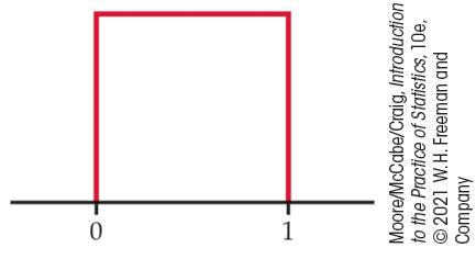
Figure 1.33 The density curve of a uniform distribution, Exercise 1.73.
-
-
1.74 Use a different range for the uniform distribution. Many random number generators allow users to specify the range of the random numbers to be produced. Suppose that you specify that the outcomes are to be distributed uniformly between 0 and 5. Then the density curve of the outcomes has constant height between 0 and 5 and height 0 elsewhere.
-
What is the height of the density curve between 0 and 5? Draw a graph of the density curve.
-
Use your graph from part (a) and the fact that areas under the curve are proportions of outcomes to find the proportion of outcomes that are more than 2.
-
Find the proportion of outcomes that lie between 2.5 and 3.0.
-
-
1.75 Find the mean, the median, and the quartiles. What are the mean and the median of the uniform distribution in Figure 1.33? What are the quartiles?
-
1.76 Three density curves. Figure 1.34 displays three density curves, each with three points marked on it. At which of these points on each curve do the mean and the median fall?
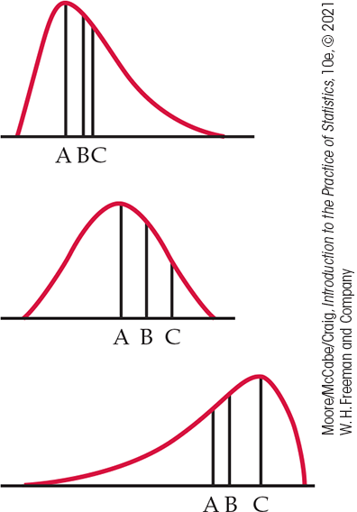
Figure 1.34 Three density curves, Exercise 1.76.
-
 1.77 Use the Normal Curve applet.
Use the Normal Curve applet for the standard Normal
distribution to say how many standard deviations above and below
the mean the quartiles of any Normal distribution lie.
1.77 Use the Normal Curve applet.
Use the Normal Curve applet for the standard Normal
distribution to say how many standard deviations above and below
the mean the quartiles of any Normal distribution lie.
-
1.78 Use the Normal Curve applet. The
68–95–99.7 rule for Normal distributions is a useful
approximation. You can use the Normal Curve applet on the
text website to see how accurate the rule is. Drag one flag
across the other so that the applet shows the area under the
curve between the two flags.
-
Place the flags one standard deviation on either side of the mean. What is the area between these two values? What does the 68–95–99.7 rule say this area is?
-
Repeat for locations two and three standard deviations on either side of the mean. Again compare the 68–95–99.7 rule with the area given by the applet.
-
-
1.79 Find some proportions. Using either software or Table A, find the proportion of observations from a standard Normal distribution that satisfies each of the following statements. In each case, sketch a standard Normal curve and shade the area under the curve that is the answer to the question.
-
-
1.80 Find more proportions. Using either software or Table A, find the proportion of observations from a standard Normal distribution for each of the following events. In each case, sketch a standard Normal curve and shade the area representing the proportion.
-
-
1.81 Find some values of z. Find the value
-
68% of the observations fall below
-
75% of the observations fall above
-
-
1.82 Find more values of z illustrate the result with a sketch. The variable
-
Find the number
-
Find the number
-
-
1.83 Find some values of z. The Wechsler Adult Intelligence Scale (WAIS) is the most common IQ test. The scale of scores is set separately for each age group, and the scores are approximately Normal, with mean 100 and standard deviation 15. People with WAIS scores below 70 are considered developmentally disabled when, for example, applying for Social Security disability benefits. What percent of adults are developmentally disabled by this criterion?
-
1.84 High IQ scores. Refer to the previous exercise, The organization MENSA, which calls itself “the high-IQ society,” requires a WAIS score of 130 or higher for membership. What percent of adults would qualify for membership?
There are two major tests of readiness for college, the ACT and the SAT. ACT scores are reported on a scale from 1 to 36. The distribution of ACT scores is approximately Normal, with mean
-
1.85 Compare an SAT score with an ACT score. Jessica scores 1240 on the SAT. Ashley scores 28 on the ACT. Assuming that both tests measure the same thing, who has the higher score? Report the
-
1.86 Make another comparison. Joshua scores 14 on the ACT. Anthony scores 690 on the SAT. Assuming that both tests measure the same thing, who has the higher score? Report the
-
1.87 Find the ACT equivalent. Jorge scores 1400 on the SAT. Assuming that both tests measure the same thing, what score on the ACT is equivalent to Jorge’s SAT score?
-
1.88 Find the SAT equivalent. Alyssa scores 32 on the ACT. Assuming that both tests measure the same thing, what score on the SAT is equivalent to Alyssa’s ACT score?
-
1.89 Find an SAT percentile. Reports on a student’s ACT or SAT results usually give the percentile as well as the actual score. The percentile is just the cumulative proportion stated as a percent: the percent of all scores that were lower than or equal to this one. Renee scores 1360 on the SAT. What is her percentile?
-
1.90 Find an ACT percentile. Reports on a student’s ACT or SAT results usually give the percentile as well as the actual score. The percentile is just the cumulative proportion stated as a percent: the percent of all scores that were lower than or equal to this one. Joshua scores 21 on the ACT. What is his percentile?
-
1.91 How high is the top 15%? What SAT scores make up the top 15% of all scores?
-
1.92 How low is the bottom 15%? What SAT scores make up the bottom 15% of all scores?
-
1.93 Find the ACT quintiles. The quintiles of any distribution are the values with cumulative proportions 0.20, 0.40, 0.60, and 0.80. What are the quintiles of the distribution of ACT scores?
-
1.94 Find the SAT quartiles. The quartiles of any distribution are the values with cumulative proportions 0.25 and 0.75. What are the quartiles of the distribution of SAT scores?
-
1.95 Do you have enough “good cholesterol”? High-density lipoprotein (HDL) is sometimes called the “good cholesterol” because high values are associated with a reduced risk of heart disease. According to the American Heart Association, people over the age of 20 years should have at least 40 milligrams per deciliter (mg/dl) of HDL cholesterol.33 U.S. women aged 20 and over have a mean HDL of 55 mg/dl with a standard deviation of 15.5 mg/dl. Assume that the distribution is Normal.
-
What percent of women have low values of HDL (40 mg/dl or less)?
-
HDL levels of 60 mg/dl and higher are believed to protect people from heart disease. What percent of women have protective levels of HDL?
-
Women with more than 40 mg/dl but less than 60 mg/dl of HDL are in the intermediate range, neither very good or very bad. What proportion are in this category?
-
-
1.96 Men and HDL cholesterol. HDL cholesterol levels for men have a mean of 46 mg/dl, with a standard deviation of 13.6 mg/dl. Assume that the distribution is Normal. Answer the questions given in the previous exercise for the population of men.
-
1.97 Diagnosing osteoporosis. Osteoporosis is a condition in which the bones become brittle due to loss of minerals. To diagnose osteoporosis, an elaborate apparatus measures bone mineral density (BMD). BMD is usually reported in standardized form. The standardization is based on a population of healthy young adults. The World Health Organization (WHO) criterion for osteoporosis is a BMD 2.5 standard deviations below the mean for young adults. BMD measurements in a population of people similar in age and sex roughly follow a Normal distribution.
-
What percent of healthy young adults have osteoporosis by the WHO criterion?
-
Women aged 70 to 79 are of course not young adults. The mean BMD in this age is about
-
-
1.98 Deciles of Normal distributions. The deciles of any distribution are the 10th, 20th, . . . , 90th percentiles. The first and last deciles are the 10th and 90th percentiles, respectively.
-
What are the first and last deciles of the standard Normal distribution?
-
The weights of 9-ounce potato chip bags are approximately Normal, with mean 9.11 ounces and standard deviation 0.14 ounce. What are the first and last deciles of this distribution?
-
-
1.99 Quartiles for Normal distributions.
The quartiles of any distribution are the values with cumulative
proportions 0.25 and 0.75.
-
What are the quartiles of the standard Normal distribution?
-
Using your numerical values from (a), write an equation that gives the quartiles of the
-
-
1.100 IQR for Normal distributions.
Continue your work from the previous exercise. The interquartile
range IQR is the distance between the first and third
quartiles of a distribution.
-
What is the value of the IQR for the standard Normal distribution?
-
There is a constant
-
-
1.101 Outliers for Normal distributions.
Continue your work from the previous two exercises. The percent
of the observations that are suspected outliers according to the
-
1.102 Deciles of HDL cholesterol. The deciles of any distribution are the 10th, 20th, . . . , 90th percentiles. Refer to Exercise 1.95 where we assumed that the distribution of HDL cholesterol in U.S. women aged 20 and over is Normal with mean 55 mg/dl and standard deviation 15.5 mg/dl. Find the deciles for this distribution.
-
1.103 Longleaf pine trees. Exercise 1.56 (page 46) gives the diameter at breast height (DBH) for 40 longleaf pine trees from the Wade Tract in Thomas County, Georgia. Make a Normal quantile plot for these data and write a short paragraph interpreting what it describes.

-
1.104 Potassium from potatoes. Refer to Exercise 1.15 (page 22), where you used s stemplot to examine the potassium absorption of a group of 27 adults who ate a controlled diet that included 40 mEq of potassium from potatoes for five days. In Exercise 1.33 (page 43), you compared the stemplot, the histogram, and the boxplot as graphical summaries of this distribution.

-
Generate these three graphical summaries.
-
Make a Normal quantile plot and interpret it.
-
-
1.105 Potassium from a supplement. Refer to Exercise 1.16 (page 22), where you used a stemplot to examine the potassium absorption of a group of 29 adults who ate a controlled diet that included 40 mEq of potassium from a supplement for five days. In Exercise 1.34 (page 43), you compared the stemplot, the histogram, and the boxplot as graphical summaries of this distribution.

-
Generate these three graphical summaries.
-
Make a Normal quantile plot and interpret it.
-