2.3 Correlation in Chapter 2 Looking at Data

2.3 Correlation

A scatterplot displays the form, direction, and strength of the relationship between two quantitative variables. Linear (straight-line) relations are particularly important because a straight line is a simple pattern that is quite common.

We say a linear relationship is strong if the points lie close to a straight line and weak if they are widely scattered about a line. Our eyes, however, are not the best judges of how strong a relationship is. The two scatterplots in Figure 2.14 depict exactly the same data, but the lower plot is in an expanded field of possible values. The lower plot seems to show a stronger relationship.

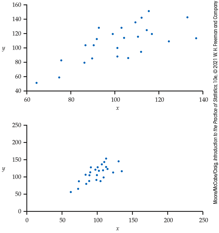
Two example scatterplots display the same data, but with different scales on their axes. — Figure 2.14 Two scatterplots of the same data. The linear pattern in the lower plot appears stronger because of the surrounding open space.

Our eyes can be fooled by changing the plotting scales or the amount of white space around the cloud of points in a scatterplot.¹⁶ We need to follow our strategy for data analysis by using a numerical measure to supplement the graph. Correlation is the measure we use.

The correlation r

Data set icon for Vtm.

We have data on variables x and y for n cases. Think, for example, of measuring height and weight of n people, including ourselves. We could then have x1 and y1 be your height and your weight, x2 and y2 be my height and my weight, and so on. The ith individual’s height xi goes with weight yi. It is these pairs of values that are used in calculating the correlation.

Correlation

The correlation measures the direction and strength of the linear relationship between two quantitative variables. Correlation is usually written as r.

Suppose that we have data on variables x and y for n individuals. The means and standard deviations of the two variables are x¯ and sx for the x-values and y¯ and sy for the y-values. The correlation r between x and y is

r=1n−1∑ (xi−x¯sx)(yi−y¯sy)

Correlations have values between −1 and 1.

As always, the summation sign ∑ means “add these terms up.” The formula for the correlation r is a bit complex. It helps us see what correlation is but is not convenient for actually calculating r. In practice, you should use software or a calculator that computes r from the values of x and y pairs.

The formula for r begins by standardizing the observations. Going back to our height and weight example, suppose that x is height in centimeters and y is weight in kilograms. Then x¯ and sx are the mean and standard deviation of the n heights, both in centimeters. The value

xi−x¯sx

is the standardized height of the ith person. A standardized value, or z-score, says how many standard deviations above or below the mean a value lies. This means standardized values have no units. For this example, this means the standardized heights are no longer measured in centimeters. If we also standardize the weights, then these two variables are now on a comparable scale. The correlation r is the average of the products of the standardized height and the standardized weight for the n people.

Example 2.19 Correlation for laundry detergents.

Figure 2.3 (page 80) gives the scatterplot of rating versus price per load for 52 laundry detergents. Software gives the value of the correlation as 0.21. A straight line is included to help us evaluate the form of the relationship. The relationship is positive and approximately linear but very weak. The value of the correlation is very low, supporting the graphical summary that shows a weak relationship.

Example 2.20 Correlation is not always a useful numerical summary.

Figure 2.1 (page 78) gives the scatterplot for the laundry detergent data with the outlier included. The major feature in the plot is the outlier, which has a somewhat average rating but a price that is about twice as much as the next most expensive detergent. The correlation measures the direction and strength of a linear relationship, so it is not a very useful numerical summary for this relationship.

Figure 2.6 (page 82) is a scatterplot of calcium retention versus calcium intake. The relationship is clearly curved where retention levels off at higher levels of intake. The correlation is not a good numerical summary for this relationship.

Check-in

2.11 Laundry detergents. Example 2.9 (page 77) describes data on the rating and price per load for 53 laundry detergents. Use software to show that the correlation between rating and price is the same as the correlation between price and rating. Report the correlation with four digits after the decimal.
2.12 Change the units. Refer to the previous Check-in question. Express the price per load in dollars.
1. Is the transformation from cents to dollars a linear transformation? Explain your answer.
2. Compute the correlation between rating and price per load expressed in dollars.
3. How does the correlation that you computed in part (b) compare with the one you computed in the previous Check-in question?
4. What can you say in general about the effect of changing units using linear transformations on the size of the correlation?

Properties of correlation

The formula for correlation helps us see that r is positive when there is a positive association between the variables. Height and weight, for example, have a positive association. People who are above average in height tend to also be above average in weight. Both the standardized height and the standardized weight for such a person are positive. People who are below average in height tend also to have below-average weight. Then both standardized height and standardized weight are negative. In both cases, the products in the formula for r are mostly positive, so r is positive. In the same way, we can see that r is negative when the association between x and y is negative. More detailed study of the formula gives more detailed properties of r.

Here is what you need to know to interpret correlation:

Correlation makes no use of the distinction between explanatory and response variables. It makes no difference which variable you call x and which you call y in calculating the correlation.
Correlation requires that both variables be quantitative. For example, we cannot calculate a correlation between the incomes of a group of people and what city they live in because city is a categorical variable.
Because r uses the standardized values of the observations, r does not change when we change the units of measurement (a linear transformation) of x, y, or both. Measuring height in inches rather than centimeters and weight in pounds rather than kilograms does not change the correlation between height and weight. The correlation r itself has no unit of measurement; it is just a number.
Positive r indicates positive association between the variables, and negative r indicates negative association.
The correlation r is always a number between −1 and 1. Values of r near 0 indicate a very weak linear relationship. The strength of the relationship increases as r moves away from 0 toward either −1 or 1. Values of r close to −1 or 1 indicate that the points lie close to a straight line.
Correlation measures the strength of only the linear relationship between two variables. Correlation does not describe curved relationships between variables, no matter how strong they are.

Like the mean and standard deviation, the correlation is not resistant: r is strongly affected by a few outlying observations. Use r with caution when outliers appear in the scatterplot.

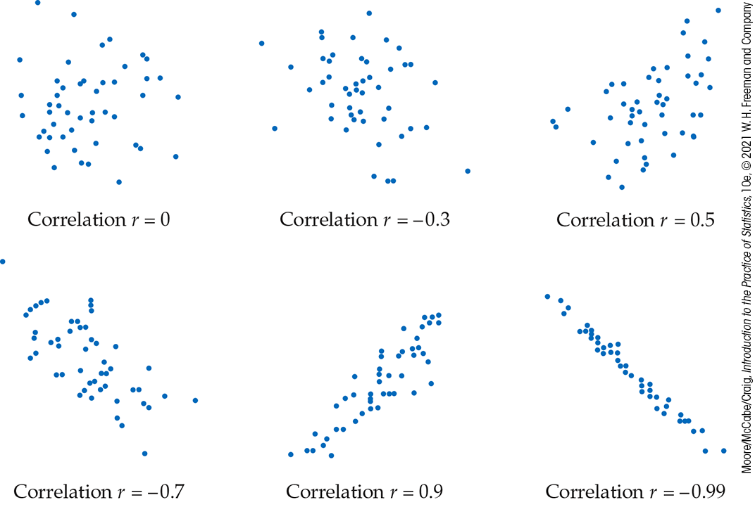
The scatterplots in Figure 2.15 illustrate how values of r closer to 1 or −1 correspond to stronger linear relationships. To make the essential meaning of r clear, the standard deviations of both variables in these plots are equal, and the horizontal and vertical scales are the same. In general, it is not so easy to guess the value of r from the appearance of a scatterplot. Remember that changing the plotting scales in a scatterplot may mislead our eyes, but it does not change the standardized values of the variables and, therefore, cannot change the correlation. To explore how extreme observations can influence r, use the Correlation and Regression applet available on the text website. Also, see Exercises 2.44 and 2.45 (pages 97–98). Applet

Six scatterplots illustrate different correlations. — Figure 2.15 How the correlation r measures the direction and strength of a linear association.

Each scatterplot shows a cluster of 40 points, each with a different correlation. For correlation r = 0, the cluster is scattered high and wide, with no discernable pattern. For r = negative 0.3, the cluster is wide and loose, but with a slight, downward diagonal pattern from left to right. For r = 0.5, the cluster rises in a loose diagonal pattern from left to right. For r = negative 0.7, the cluster falls in a slightly tighter diagonal pattern from left to right. For r = 0.9, the points rise in a tight diagonal cluster from left to right. For r = negative 0.99, the cluster falls in a very tight, nearly straight diagonal pattern from left to right.

Finally, remember that correlation is not a complete description of two-variable data, even when the relationship between the variables is linear. You should give the means and standard deviations of both x and y along with the correlation. (Because the formula for correlation uses the means and standard deviations, these measures are the proper choices to accompany a correlation.) Conclusions based on correlations alone may require rethinking in the light of a more complete description of the data.

Example 2.21 Scoring of figure skating in the Olympics.

Until a scandal at the 2002 Olympics brought change, figure skating was scored by judges on a scale from 0.0 to 6.0. The scores were often controversial. We have the scores awarded by two judges, Pierre and Elena. How well do they agree? The correlation between their scores is r=0.9. But the mean of Pierre’s scores is 0.8 point lower than Elena’s mean.

These facts in Example 2.21 do not contradict each other. They are simply different kinds of information. The mean scores show that Pierre awards lower scores than Elena. But because Pierre gives every skater a score about 0.8 point lower than Elena, the correlation remains high. Adding the same number to all values of either x or y does not change the correlation. If both judges score the same skaters, the competition is scored consistently because Pierre and Elena agree on which performances are better than others. The high r shows their agreement. But if Pierre scores some skaters and Elena others, we must add 0.8 point to Pierre’s scores to arrive at a fair comparison.

Section 2.3 SUMMARY

The correlation r measures the direction and strength of the linear (straight-line) association between two quantitative variables x and y. It has no unit of measurement.
Correlation indicates the direction of a linear relationship by its sign: r>0 for a positive association and r<0 for a negative association.
Correlation always satisfies −1≤r≤1 and indicates the strength of a relationship by how close it is to −1 or 1.
Correlation ignores the distinction between explanatory and response variables. The value of r is not affected by changes in the unit of measurement of either variable.
While scatterplots give a full graphical summary of the relationship between two variables, it can be hard to see the form of the relationship. The correlation can give a better description of the relationship, but it is only meaningful for linear relationships, and is not resistant to outliers (which can greatly change the value of r).

Now that you have completed this section, you will be able to:

Use a correlation to describe the direction and strength of a linear relationship between two quantitative variables. Review Example 2.19 (page 93) and try Exercise 2.31.
Identify situations in which the correlation is not a good measure of association between two quantitative variables. Review Example 2.20 (page 93) and try Exercise 2.47.
Identify the roles of the correlation, a numerical summary, and the scatterplot, a graphical summary, for describing the relationship between two quantitative variables. Review Example 2.19 (page 93) and try Exercise 2.33.

Section 2.3 EXERCISES

2.28 What’s wrong? Explain what is wrong with each of the following:
1. A correlation of 2.0 indicates a very strong positive relationship.
2. When reporting a correlation, you should always give its units.
3. The correlation between two quantitative variables is always positive.
4. Ashley obtains the blood pressure of 10 students from her dorm, and Madison obtains a stress score of 10 students from her dorm. A scatterplot of these two variables will help to explain the correlation between them.
2.29 Interpret some correlations. For each of the following correlations, describe the relationship between the two quantitative variables in terms of the direction and the strength of the linear relationship.
1. r=0.01.
2. r=0.8.
3. r=−0.8.
4. r=−0.2.
2.30 Blueberries and anthocyanins. In Exercise 2.8 (page 88), you examined the relationship between Antho4 and Antho3, two anthocyanins found in blueberries.
1. Find the correlation between these two anthocyanins.
2. Look at the scatterplot for these data that you made in part (a) of Exercise 2.8 (or make one if you did not do that exercise). Is the correlation a good numerical summary of the graphical display in the scatterplot? Explain your answer.
3. Does the size of the correlation suggest that the amounts of these two anthocyanins is approximately equal in these blueberries? Explain why or why not.
2.31 Blueberries and anthocyanins with logs. In Exercise 2.9 (page 88), you examined the relationship between Antho4 and Antho3, two anthocyanins found in blueberries, using logs for both variables. Answer the questions in the previous exercise for the variables transformed in this way.
2.32 Fuel consumption. In Exercise 2.11 (page 88), you used a scatterplot to examine the relationship between CO2 emissions and highway fuel consumption for 502 vehicles that use regular fuel. Find the correlation between these two variables. Use the scatterplot and the correlation to describe the relationship.
2.33 Fuel consumption for different types of vehicles. In Exercise 2.13 (page 89), you examined the relationship between CO2 emissions and highway fuel consumption for 1045 vehicles that use four different types of fuel. Find the correlations between CO2 and highway fuel consumption for each of these four categories of vehicle. Summarize your results and explain the similarities and differences in the relationships among the four types of fuel.

2.34 Strong association but no correlation. Here is a data set that illustrates an important point about correlation:

X	45	55	65	75	85
Y	30	50	70	50	30

Make a scatterplot of Y versus X.
Describe the relationship between Y and X. Is it weak or strong? Is it linear?
Find the correlation between Y and X.
What important point about correlation does this exercise illustrate?

2.35 Bone strength. Exercise 2.14 (page 89) gives the bone strengths of the dominant and the nondominant arms of 15 men who were controls in a study.
1. Find the correlation between the bone strength of the dominant arm and the bone strength of the nondominant arm.
2. Look at the scatterplot for these data that you made in part (a) of Exercise 2.14 (or make one if you did not do that exercise). Is the correlation a good numerical summary of the graphical display in the scatterplot? Explain your answer.
2.36 Bone strength for baseball players. Refer to the previous exercise. Similar data for baseball players are given in Exercise 2.15 (page 89). Answer parts (a) and (b) of the previous exercise for these data.
2.37 Student ratings of teachers. A college newspaper interviews a psychologist about student ratings of the teaching of faculty members. The psychologist says, “The evidence indicates that the correlation between the research productivity and teaching rating of faculty members is close to zero.” The paper reports this as “Professor McDaniel said that good researchers tend to be poor teachers, and vice versa.” Explain why the paper’s report is wrong. Write a statement in plain language (without using the word “correlation”) to explain the psychologist’s meaning.
2.38 Decay of a radioactive element. Data for an experiment on the decay of barium-137m is given in Exercise 2.22 (page 90).
1. Find the correlation between the radioactive counts and the time after the start of the first counting period.
2. Does the correlation give a good numerical summary of the relationship between these two variables? Explain your answer.
2.39 Decay in the log scale. Refer to the previous exercise and to Exercise 2.23 (page 90), where the counts were transformed by a log.
1. Find the correlation between the log counts and the time after the start of the first counting period.
2. Does the correlation give a good numerical summary of the relationship between these two variables? Explain your answer.
3. Compare your results for this exercise with those from the previous exercise.
2.40 Brand names and generic products.
1. If a store always prices its generic “store brand” products at 80% of the brand name products’ prices, what would be the correlation between the prices of the brand name products and the store brand products? (Hint: Draw a scatterplot for several prices.)
2. If the store always prices its generic products $2 less than the corresponding brand name products, then what would be the correlation between the prices of the brand name products and the store brand products?
2.41 Alcohol and calories in beer. Figure 2.12 (page 90) gives a scatterplot of the calories versus percent alcohol for 160 brands of domestic beer.
1. Compute the correlation for these data.
2. Does the correlation do a good job of describing the direction and strength of this relationship? Explain your answer.
2.42 Alcohol and calories in beer revisited. Refer to the previous exercise. The data that you used to compute the correlation include an outlier.
1. Remove the outlier and recompute the correlation.
2. Write a short paragraph about the possible effects of outliers on a correlation, using this example to illustrate your ideas.
2.43 Compare domestic with imported. In Exercise 2.21 (page 90), you compared domestic beers with imported beers with respect to the relationship between calories and percent alcohol. In that exercise, you used scatterplots to make the comparison. Compute the correlations for these two categories of beer and write a new summary of the comparison, using correlations in addition to the scatterplots.
2.44 Use the applet. Go to the Correlation and Regression applet. Click on the scatterplot to create a group of 10 points in the lower-left corner of the scatterplot with a strong straight-line positive pattern (correlation about 0.9).
1. Add one point at the upper right that is in line with the first 10. How does the correlation change?
2. Drag this last point down until it is opposite the group of 10 points. How small can you make the correlation? Can you make the correlation negative? A single outlier can greatly strengthen or weaken a correlation. Always plot your data to check for outlying points.
2.45 Use the applet. You are going to use the Correlation and Regression applet to make different scatterplots with 10 points that have correlation close to 0.9. Many patterns can have the same correlation. Always plot your data before you trust a correlation.
1. Stop after adding the first two points. What is the value of the correlation? Why does it have this value no matter where the two points are located?
2. Make a lower-left to upper-right pattern of 10 points with correlation about r=0.9. (You can drag points up or down to adjust r after you have 10 points.) Make a rough sketch of your scatterplot.
3. Make another scatterplot, this time with 9 points in a vertical stack at the left of the plot. Add one point far to the right and move it until the correlation is close to 0.9. Make a rough sketch of your scatterplot.
4. Make yet another scatterplot, this time with 10 points in a curved pattern that starts at the lower left, rises to the right, then falls again at the far right. Adjust the points up or down until you have a quite smooth curve with correlation close to 0.8. Make a rough sketch of this scatterplot also.

2.46 An interesting set of data. Make a scatterplot of the following data:

x	1	2	3	4	10	10
y	1	3	3	5	1	11

Verify that the correlation is about 0.5. What feature of the data is responsible for reducing the correlation to this value despite a strong straight-line association between x and y in most of the observations?

2.47 Internet use and babies. Figure 2.13 (page 90) is a scatterplot of the number of births per 1000 people versus Internet users per 100 people for 106 countries. In Exercise 2.24 (page 90), you described this relationship.
1. Make a plot of the data similar to Figure 2.13 and report the correlation.
2. Is the correlation a good numerical summary for this relationship? Explain your answer.
2.48 What’s wrong? Explain what is wrong with each of the following:
1. There is a high correlation between the age of American workers and their occupation.
2. We found a high correlation (r=1.19) between students’ ratings of faculty teaching and ratings made by other faculty members.
3. The correlation between the sex of a group of students and the color of their cell phone was r=0.23.