2.5 Cautions about Correlation and Regression in Chapter 2 Looking at Data

2.5 Cautions about Correlation and Regression

When you complete this section, you will be able to:

Identify situations where using a regression equation for prediction would not be accurate because of extrapolation.
Calculate the residuals for a set of data using the equation of the least-squares regression line and the observed values of the explanatory variable.
Use a plot of the residuals versus the explanatory variable to assess the fit of a regression line.
Identify outliers and influential observations by examining scatterplots and residual plots.
Identify lurking variables that can influence the interpretation of relationships between two variables.
Explain the difference between association and causality when interpreting the relationship between two variables.

Correlation and regression are among the most common statistical tools. They are used in more elaborate form to study relationships among many variables, a situation in which we cannot see the essentials by studying a single scatterplot. We need a firm grasp of the use and limitations of these tools, both now and as a foundation for more advanced statistics.

Extrapolation

Associations for variables can be trusted only for the range of values for which data have been collected. Even a very strong relationship may not hold outside the data’s range.

Example 2.31 Predicting the number of Target stores.

Here are data on the number of Target stores in operation at the end of each year in the early 1990s, in 2008, in 2014, and in 2018:²¹

Year (x)	1990	1991	1992	1993	2008	2014	2018
Stores (y)	420	463	506	554	1682	1916	1829

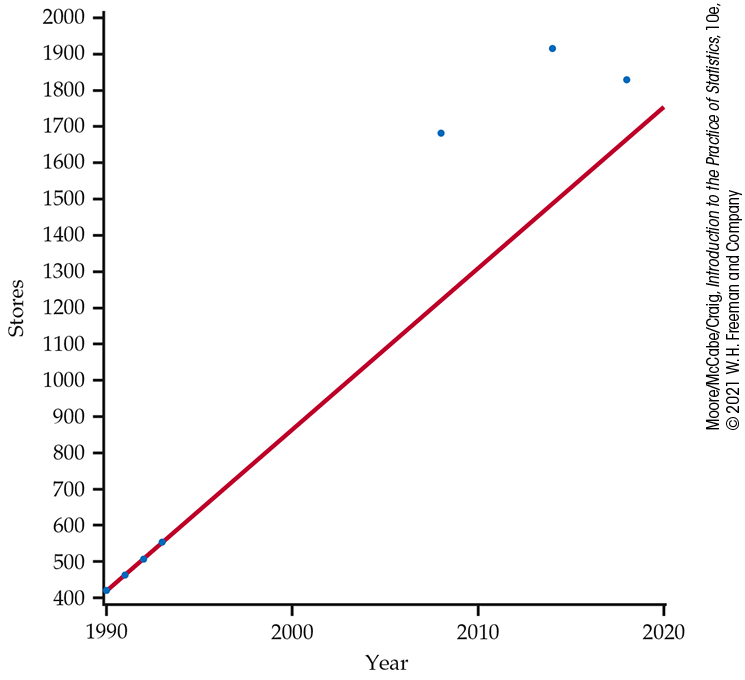
A plot of these data is given in Figure 2.23. The data for 1990 through 1993 lie almost exactly on a straight line. The equation of the line is y=−88, 136+44.5x and r2=0.9992. We know that 99.92% of the variation in the number of stores is explained by year for these years. The equation predicts 1220 stores for 2008, but the actual number of stores is much higher, 1682. It predicts 1487 for 2014 and 1665 for 2018. These predictions are very poor because the very strong linear trend evident in the early 1990s did not continue.

A data set icon of stores versus year. — Figure 2.23 Plot of the number of Target stores versus year with the least-squares regression line calculated using data from 1990, 1991, 1992, and 1993, Example 2.31. The poor fits to the number of stores in 2008, 2014, and 2018 illustrate the dangers of extrapolation.

Making predictions far beyond the range for which data have been collected is called extrapolation. Such predictions can’t be trusted. Few relationships are linear for all values of x. It is risky to stray far from the range of x-values that actually appear in your data.

Check-in

2.20 Would you use the regression equation to predict? Refer to the scatterplot of the relationship between MI and IDI with the least-squares regression line in Figure 2.16 (page 99). Consider the following values for MI: −$10, $2, $20, $50, $200. For each, decide whether you would use the least-squares regression equation to predict IDI or whether you would be concerned that the prediction would not be trustworthy because of extrapolation. Give reasons for your answers.

Residuals

Data set icon for Vtm.

A regression line is a mathematical model for the overall pattern of a linear relationship between an explanatory variable and a response variable. Deviations from the overall pattern are also important. In the regression setting, we see deviations by looking at the scatter of the data points about the regression line. The vertical distances from the points to the least-squares regression line are as small as possible in the sense that they have the smallest possible sum of squares. Because they represent “leftover” variation in the response after fitting the regression line, these distances are formally called residuals.

Example 2.32 Education spending and population.

Figure 2.24 is a scatterplot showing education spending versus the population for the 50 states. Included on the scatterplot is the least-squares regression line. The points for the states with large values for both variables—California, Texas, Florida, and New York—are marked individually.

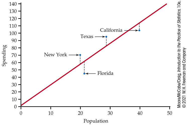
A scatterplot of spending versus population. — Figure 2.24 Scatterplot of spending on education versus the population for the 50 U.S. states, with the least-squares line and selected points labeled, Example 2.32.

The equation of the least-squares regression line is y^=1.38017+2.82654x, where y^ represents education spending and x represents the population of the state.

Let’s look carefully at the data for California, y=103.7 and x=39.8. The predicted education spending for a state with 39.8 million people is

y^=1.38017+2.82654(39.8)=113.88

The residual for California is the difference between the observed spending (y) and this predicted value:

residual=y−y^=103.70−113.88=−10.18

California spends $10.18 million less on education than the least-squares regression line predicts. On the scatterplot, the residual for California is shown as a dashed vertical line between the actual spending and the least-squares regression line. The residual appears below the line because it is negative.

Check-in

2.21 Residual for Texas. Refer to Example 2.32. Texas spent $95.3 million on education and has a population of 28.7 million people.
1. Find the predicted education spending for Texas.
2. Find the residual for Texas.
3. Which state, California or Texas, has a greater deviation from the least-squares regression line?

There is a residual for each data point. Finding the residuals with a calculator is a bit unpleasant because you must first find the predicted response for every x. Statistical software gives you the residuals all at once.

Because the residuals show how far the data fall from our regression line, examining the residuals helps us assess how well the line describes the data. Although residuals can be calculated from any model fitted to data, the residuals from the least-squares regression line have a special property: the mean of the least-squares residuals is always zero. When we compute with real data, the residuals are generally rounded off, so the sum will be very small but not always exactly zero.

Check-in

2.22 Sum the education spending residuals. In addition to the variables described in Example 2.12 (page 81), the EDSPEND data set contains the residuals rounded to two places after the decimal. Find the sum of these residuals. Is the sum exactly zero? If not, explain why.

As usual, when we perform statistical calculations, we prefer to display the results graphically. We can do this for the residuals.

Example 2.33 Residual plot for education spending.

Figure 2.25 gives the residual plot for the education spending data. The horizontal line at zero in the plot helps orient us.

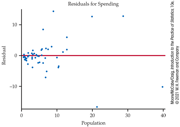
A residual plot of spending. — Figure 2.25 Residual plot for the education spending data, Example 2.33.

Check-in

2.23 Identify the four states. In Figure 2.24 (page 115), four states are identified by name: California, Texas, Florida, and New York. The dashed lines in the plot represent the residuals.
1. Sketch a version of Figure 2.24 or generate your own plot using the EDSPEND data file. Include the points for all states. Write in the names of the states California, Texas, Florida, and New York on your plot.
2. Explain how you were able to identify these four points on your sketch.

If the least-squares regression line captures the overall relationship between x and y, the residuals should have no systematic pattern. The residual plot will look something like the pattern in Figure 2.26(a). That plot shows a scatter of points about the fitted line, with no unusual individual observations or systematic change as x increases. Here are some things to look for when you examine a residual plot:

A curved pattern, which shows that the relationship is not linear. Figure 2.26(b) is a simplified example. A straight line is not a good summary for such data.
Increasing or decreasing spread about the line as x increases. Figure 2.26(c) is a simplified example. Prediction of y will be less precise for larger x in that example.
Individual points with large residuals, which are outliers in the vertical (y) direction because they lie far from the line that describes the overall pattern.
Individual points that are extreme in the x direction. Such points may or may not have large residuals, but they can be very important. We address such points next.

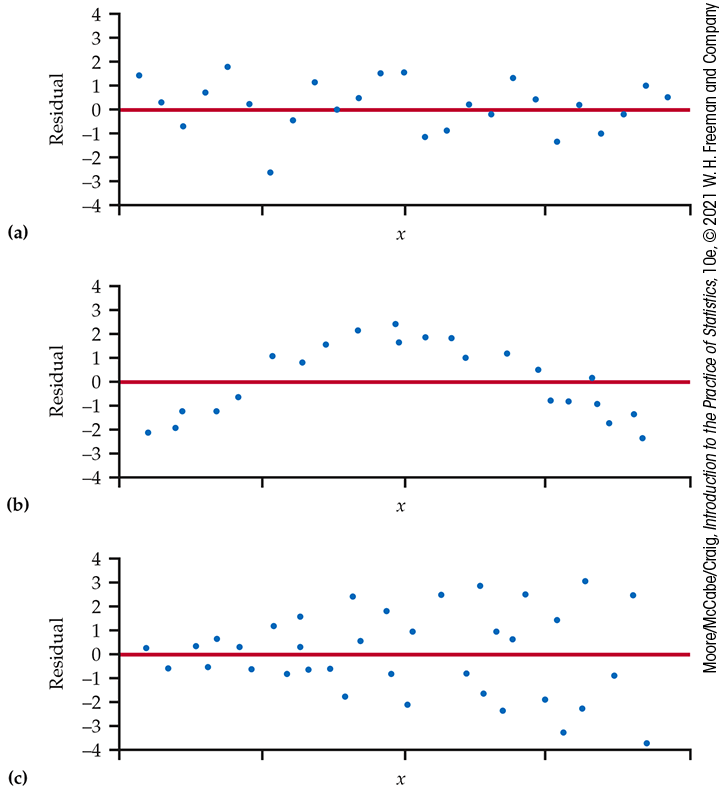
Three residual plots showing three different patterns. — Figure 2.26 Idealized patterns in plots of least-squares residuals. Plot (a) indicates that the regression line fits the data well. The data in plot (b) have a curved pattern, so a line is not a good fit. The response variable y in plot (c) has more spread for larger values of the explanatory variable x, so predictions will be less accurate when x is large.

The distribution of the residuals

When we compute the residuals, we are creating a new quantitative variable for our data set. Each case has a value for this variable. It is natural to ask about the distribution of this variable. We already know that the mean is zero, but we can use the methods we learned in Chapter 1 to examine other characteristics of the distribution. As we will see in Chapter 10, a question of interest with respect to residuals is whether they are approximately Normal. Recall that we used Normal quantile plots to address this issue.

Example 2.34 Are the residuals approximately Normal?

Figure 2.27 gives the Normal quantile plot for the residuals in our education spending example. The distribution of the residuals is not Normal. Most of the points are close to a line in the center of the plot, but there appear to be four outliers: one with a negative residual and three with positive residuals.

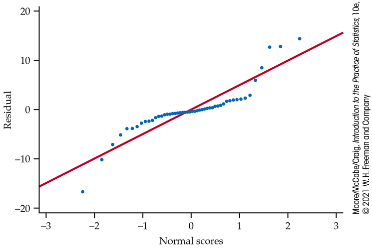
A normal quantile plot of education spending. — Figure 2.27 Normal quantile plot of the residuals for the education spending regression, Example 2.34.

Take a look at the plot of the data with the least-squares regression line in Figure 2.5 (page 82). Note that you can see the same four points in this plot. If we eliminated these states from our data set, the remaining residuals would be approximately Normal. However, there is nothing wrong with the data for these four states. To account for them, a complete analysis of the data should include a statement that they are somewhat extreme relative to the distribution of the other states.

Outliers and influential observations

When you look at scatterplots and residual plots, look for striking individual points as well as for an overall pattern. Here is an example of data that contain some unusual cases.

Example 2.35 Diabetes and blood sugar.

People with diabetes must manage their blood sugar levels carefully. They measure their fasting plasma glucose (FPG) with a glucose meter. Another measurement, made at regular medical checkups, is called HbA1c. This is roughly the percent of red blood cells that have a glucose molecule attached. It measures average exposure to glucose over a period of several months.

This diagnostic test is becoming widely used and is sometimes called A1c by health care professionals. Table 2.2 gives data on both HbA1c and FPG for 18 diabetics five months after they completed a diabetes education class.²²

Table 2.2 Two measures of glucose level in diabetics
Subject	HbA1c (%)	FPG (mg/dl)	Subject	HbA1c (%)	FPG (mg/dl)	Subject	HbA1c (%)	FPG (mg/dl)
1	6.1	141	7	7.5	96	13	10.6	103
2	6.3	158	8	7.7	78	14	10.7	172
3	6.4	112	9	7.9	148	15	10.7	359
4	6.8	153	10	8.7	172	16	11.2	145
5	7.0	134	11	9.4	200	17	13.7	147
6	7.1	95	12	10.4	271	18	19.3	255

Because both FPG and HbA1c measure blood glucose, we expect a positive association. The scatterplot in Figure 2.28(a) shows a surprisingly weak relationship, with correlation r=0.8419. The line on the plot is the least-squares regression line for predicting FPG from HbA1c. Its equation is

y^=66.4+10.41x

It appears that one-time measurements of FPG can vary quite a bit among people with similar long-term levels, as measured by HbA1c. This is why A1c is an important diagnostic test.

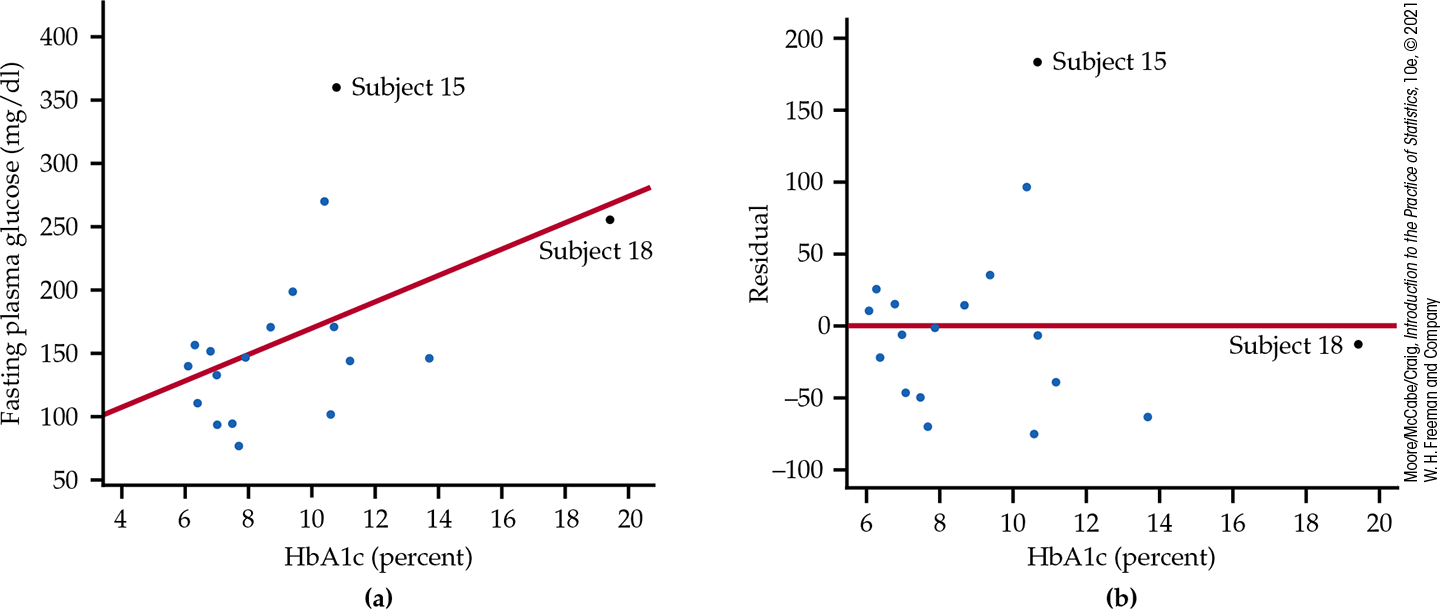
A scatterplot and residual plot of H b A 1 c percentages. — Figure 2.28 (a) Scatterplot of fasting plasma glucose against HbA1c (which measures long-term blood glucose), with the least-squares regression line, Example 2.35. (b) Residual plot for the regression of fasting plasma glucose on HbA1c. Subject 15 is an outlier in fasting plasma glucose. Subject 18 is an outlier in HbA1c that may be influential but does not have a large residual.

Scatterplot a plots fasting plasma glucose milligrams per deciliter on the vertical axis, ranging from 50 to 400 in increments of 50, versus H b A 1 c in percent on the horizontal axis, ranging from 4 to 20 in increments of 2. Eighteen points are plotted in a wide, loose cluster that is slightly linear, rising from left to right between 6 and 14 on the horizontal axis and 70 and 270 on the vertical axis. Two outlying points are plotted for subject 15 at (10.5, 350) and subject 18 at (19.5, 250). A diagonal regression line rises through the center of the cluster from (4, 100) through (20, 300). Residual plot b plots residual on the vertical axis, ranging from negative 100 to 200 in increments of 50, versus H b A 1 c in percent on the horizontal axis, ranging from 6 to 20 in increments of 2. A horizontal residual line extends horizontally from 0 on the vertical axis. Eighteen points are plotted high and wide between 6 and 14 on the horizontal axis and negative 75 and 100 on the vertical axis. Two outlying points are plotted for subject 15 at (10.5, 175) and subject 18 at (19.5, negative 10). All values estimated.

Two unusual cases are marked in Figure 2.28(a). Subjects 15 and 18 are unusual in different ways. Subject 15 has dangerously high FPG and lies far from the regression line in the y direction. Subject 18 is close to the line but far out in the x direction. The residual plot in Figure 2.28(b) confirms that Subject 15 has a large residual and that Subject 18 does not.

Points that are outliers in the x direction, like Subject 18, can have a strong influence on the position of the regression line. Least-squares lines make the sum of squares of the vertical distances to the points as small as possible. A point that is extreme in the x direction with no other points near it pulls the line toward itself.

Influence is a matter of degree: How much does a calculation change when we remove an observation? It is difficult to assess influence on a regression line without actually doing the regression both with and without the suspicious observation. Although a point that is an outlier in x is often influential, if the point happens to lie close to the regression line calculated from the other observations, then its presence will move the line only a little, and the point will not be influential.

The influence of a point that is an outlier in y depends on whether there are many other points with similar values of x that hold the line in place. Figures 2.28(a) and (b) identify two unusual observations. How influential are they?

Example 2.36 Influential observations.

Subjects 15 and 18 both influence the correlation between FPG and HbA1c but in opposite directions. Subject 15 weakens the linear pattern; if we drop this point, the correlation increases from r=0.5684 to r=0.4819. Subject 18 extends the linear pattern; if we omit this subject, the correlation drops from r=0.4819 to r=0.3837.

To assess influence on the least-squares regression line, we recalculate the line, leaving out a suspicious point. Figure 2.29 shows three least-squares regression lines. The solid line is the least-squares regression line of FPG on HbA1c based on all 18 subjects. This is the same line that appears in Figure 2.28(a). The dotted line is calculated from all subjects except Subject 18. You see that point 18 does pull the line down toward itself. But the influence of Subject 18 is not very large: the dotted and solid lines are close together for HbA1c values between 6 and 14, the range of all except Subject 18.

The dashed line omits Subject 15, the outlier in y. Comparing the solid and dashed lines, we see that Subject 15 pulls the least-squares regression line up. The influence is again not large, but it exceeds the influence of Subject 18.

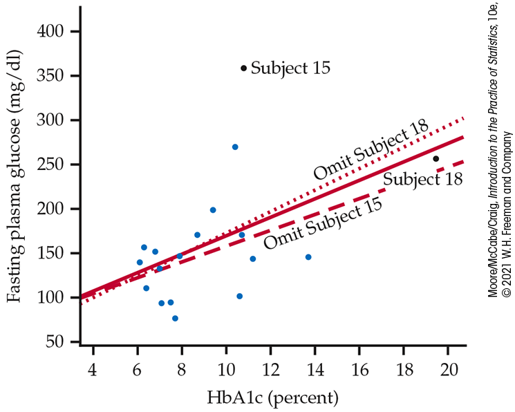
A scatterplot illustrating the effect of outliers. — Figure 2.29 Three regression lines for predicting fasting plasma glucose from HbA1c, Example 2.36. The solid line uses all 18 subjects. The dotted line leaves out Subject 18. The dashed line leaves out Subject 15. “Leaving one out” calculations are the surest way to assess influence.

The graph plots fasting plasma glucose in milligrams per deciliter on the vertical axis, ranging from 50 to 400 in increments of 50, versus H b A 1 c in percent on the horizontal axis, ranging from 4 to 20 in increments of 2. Eighteen points are plotted in a wide, loose cluster that is slightly linear, rising from left to right between 6 and 14 on the horizontal axis and 70 and 27 on the vertical axis. Two outlying points are plotted for subject 15 at (10.5, 350) and subject 18 at (19.5, 250). A regression line for all data rises diagonally through the center of the cluster from (4, 100) through (20, 270). A regression line for the data without the point for subject 15 is shallower, rising diagonally from (4, 100) through (20, 240). A regression line for the data without the point for subject 18 is steeper, rising diagonally from (4, 100) through (20, 300). All values estimated.

We did not need the distinction between outliers and influential observations in Chapter 1. A single large salary that pulls up the mean salary x¯ for a group of workers is an outlier because it lies far above the other salaries. It is also influential because the mean changes when it is removed. In the regression setting, however, not all outliers are influential. Because influential observations draw the least-squares regression line toward themselves, we may not be able to spot them by looking for large residuals.

Beware of the lurking variable

Correlation and regression are powerful tools for measuring the association between two variables and for expressing the dependence of one variable on the other. These tools must be used with an awareness of their limitations. We have seen that

Correlation measures only linear association, and fitting a straight line makes sense only when the overall pattern of the relationship is linear. Always plot your data before calculating.
Extrapolation (using a fitted model far outside the range of the data that we used to fit it) often produces unreliable predictions.
Correlation and least-squares regression are not resistant. Always plot your data and look for potentially influential points.

Another caution is even more important: caution the relationship between two variables can often be understood only by taking other variables into account. Lurking variables can make a correlation or regression misleading.

Example 2.37 Discrimination in medical treatment?

Studies show that men who complain of chest pain are more likely to get detailed tests and aggressive treatment such as bypass surgery than are women with similar complaints. Is this association between sex and treatment due to discrimination?

Perhaps not. Men and women develop heart problems at different ages—women are, on the average, between 10 and 15 years older than men. Aggressive treatments are more risky for older patients, so doctors may hesitate to recommend them.

Lurking variables—the patient’s age and condition—may explain the relationship between sex and doctors’ decisions in the studies. Here is an example of a different type of lurking variable.

Example 2.38 Gas and electricity bills.

A single-family household receives bills for gas and electricity each month. The 12 observations for a recent year are plotted with the least-squares regression line in Figure 2.30. We have arbitrarily chosen to put the electricity bill on the x axis and the gas bill on the y axis. There is a clear negative association. Does this mean that a high electricity bill causes the gas bill to be low and vice versa?

To understand the association in this example, we need to know a little more about the two variables. In this household, heating is done by gas, and cooling is done by electricity. Therefore, in the winter months, the gas bill will be relatively high and the electricity bill will be relatively low. The pattern is reversed in the summer months. The association that we see in this example is due to a lurking variable: time of year.

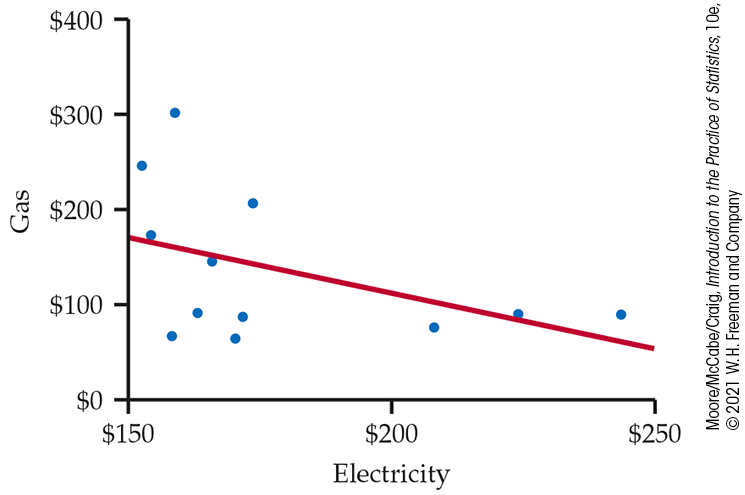
A scatterplot of gas versus electricity. — Figure 2.30 Scatterplot with least-squares regression line for predicting a household’s monthly charges for gas using its monthly charges for electricity, Example 2.38.

Correlations that are due to lurking variables are sometimes called “nonsense correlations.” The correlation is real. What is nonsense is the suggestion that the variables are directly related so that changing one of the variables causes changes in the other. The question of causation is important enough to merit separate treatment in Section 2.7. For now, just caution remember that an association between two variables x and y can reflect many types of relationships among x, y, and one or more lurking variables.

Lurking variables sometimes create a correlation between x and y, as in Examples 2.37 and 2.38. caution When you observe an association between two variables, always ask yourself if the relationship that you see might be due to a lurking variable. As in Example 2.38, time is often a likely candidate.

Beware of correlations based on averaged data

Regression or correlation studies sometimes work with averages or other measures that combine information from many individuals. For example, if we plot the average height of young children against their age in months, we will see a very strong positive association with correlation near 1. But individual children of the same age vary a great deal in height. A plot of height against age for individual children will show much more scatter and lower correlation than the plot of average height against age.

caution A correlation based on averages over many individuals is usually higher than the correlation between the same variables based on data for individuals. This fact reminds us again of the importance of noting exactly what variables a statistical study involves.

Beware of restricted ranges

The range of values for the explanatory variable in a regression can have a large impact on the strength of the relationship. For example, if we use age as a predictor of reading ability for a sample of students in the third grade, we will probably see little or no relationship. However, if our sample includes students from grades 1 through 8, we would expect to see a relatively strong relationship. We call this phenomenon the restricted-range problem.

Example 2.39 A test for job applicants.

Your company gives a test of cognitive ability to job applicants before deciding whom to hire. Your boss has asked you to use company records to see if this test really helps predict the performance ratings of employees. The restricted-range problem may make it difficult to see a strong relationship between test scores and performance ratings. The current employees were selected by a mechanism that is likely to result in scores that tend to be higher than those of the entire pool of applicants.

Beyond the Basics

Data mining

Chapters 1 and 2 of this text are devoted to the important aspect of statistics called exploratory data analysis (EDA). We use graphs and numerical summaries to examine data, searching for patterns and paying attention to striking deviations from the patterns we find. In discussing regression, we advanced to using the pattern we find (in this case, a linear pattern) for prediction.

Suppose now that we have a truly enormous database, such as all purchases recorded by the cash register scanners of a national retail chain during the past week. Surely this treasure chest of data contains patterns that might guide business decisions. If we could see clearly the types of activewear preferred in large California cities and compare the preferences of small midwestern cities—right now, not at the end of the season—we might improve profits in both parts of the country by matching stock with demand. This sounds much like EDA, and indeed it is. Exploring really large databases in the hope of finding useful patterns is called data mining. Here are some distinctive features of data mining:

When you have terabytes of data, even straightforward calculations and graphics become very time-consuming. So, efficient algorithms are very important.
The structure of the database and the process of storing the data (the fashionable term is data warehousing), perhaps by unifying data scattered across many departments of a large corporation, require careful consideration.
Data mining requires automated tools that work based on only vague queries by the user. The process is too complex to do step-by-step as we have done in EDA.

All these features point to the need for sophisticated computer science as a basis for data mining. Indeed, data mining is often viewed as a part of computer science. Yet many statistical ideas and tools—mostly tools for dealing with multidimensional data, not the sort of thing that appears in a first statistics course—are very helpful. Like many other modern developments, data mining crosses the boundaries of traditional fields of study.

Do remember that the perils we associate with blind use of correlation and regression are yet more perilous in data mining, where the fog of an immense database can prevent clear vision. Extrapolation, ignoring lurking variables, and confusing association with causation are traps for the unwary data miner.

Section 2.5 SUMMARY

Extrapolation is the use of a least-squares regression line for prediction far outside the range of the values of the explanatory variable.
You can examine the fit of a least-squares regression line by plotting the residuals, which are the differences between the observed and predicted values of y. Be on the lookout for points with unusually large residuals and also for nonlinear patterns and uneven variation about the line.
Also look for influential observations, individual points that substantially change the least-squares regression line. Influential observations are often outliers in the x direction, but they need not have large residuals.
Correlation and regression must be interpreted with caution. Plot the data to be sure that the relationship is roughly linear and to detect outliers and influential observations.
Lurking variables may explain the relationship between the explanatory and response variables. Correlation and regression can be misleading if you ignore important lurking variables.
We cannot conclude that there is a cause-and-effect relationship between two variables just because they are strongly associated. High correlation does not imply causation.
A correlation based on averages is usually higher than if we used data for individuals.

Now that you have completed this section, you will be able to:

Identify situations where using a regression equation for prediction would not be accurate because of extrapolation. Review Example 2.31 (page 114) and try Exercise 2.79.
Calculate the residuals for a set of data using the equation of the least-squares regression line and the observed values of the explanatory variable. Review Example 2.32 (page 115) and try Exercise 2.77.
Use a plot of the residuals versus the explanatory variable to assess the fit of a regression line. Review Example 2.33 (page 117) and try Exercise 2.81.
Identify outliers and influential observations by examining scatterplots and residual plots. Review Example 2.35 (page 119) and try Exercise 2.83.
Identify lurking variables that can influence the interpretation of relationships between two variables. Review Example 2.37 (page 122) and try Exercise 2.89.
Explain the difference between association and causality when interpreting the relationship between two variables. Review Example 2.38 (page 122) and try Exercise 2.91.

Section 2.5 EXERCISES

2.76 Bone strength. Exercise 2.14 (page 89) gives the bone strengths of the dominant and the nondominant arms for 15 men who were controls in a study. The least-squares regression line for these data is

dominant =2.74+(0.936× nondominant)

Here are the data for four cases:

ID	Nondominant	Dominant	ID	Nondominant	Dominant
5	12.0	14.8	7	12.3	13.1
6	20.0	19.8	8	14.4	17.5

Calculate the residuals for these four cases.

2.77 Bone strength for baseball players. Refer to the previous exercise. Similar data for baseball players is given in Exercise 2.15 (page 89). The equation of the least-squares line for the baseball players is

dominant =0.886+(1.373× nondominant)

Here are the data for the first four cases:

ID	Nondominant	Dominant	ID	Nondominant	Dominant
20	21.0	40.3	22	31.5	36.9
21	14.6	20.8	23	14.9	21.2

Calculate the residuals for these four cases.

2.78 Extrapolation for bone strength. Refer to Exercise 2.76. Would you be concerned that the least-squares regression equation would not be accurate for each of these values of nondominant arm strength: 10.0, 13.0, 16.0, 19.0, 30.0?
2.79 Extrapolation for baseball players’ bone strength. Refer to Exercise 2.76. Would you be concerned that the least-squares regression equation would not be accurate for each of these values of nondominant arm strength: 10.0, 13.0, 16.0, 19.0, 30.0?

2.80 Least-squares regression for radioactive decay. Refer to Exercise 2.22 (page 90) for the data on radioactive decay of barium-137m. Here are the data:

Time	1	3	5	7
Count	578	317	203	118

Using the least-squares regression equation

count =602.8−(74.7× time)

and the observed data, find the residuals for the counts.
Plot the residuals versus time.
Write a short paragraph assessing the fit of the least-squares regression line to these data, based on your interpretation of the residual plot.

2.81 Least-squares regression for the log counts. Refer to Exercise 2.23 (page 90), where you analyzed the radioactive decay of barium-137m data using log counts. Here are the data:

Time	1	3	5	7
Log count	6.35957	5.75890	5.31321	4.77068

Using the least-squares regression equation

log count =6.593−(0.2606× time)

and the observed data, find the residuals for the counts.
Plot the residuals versus time.
Write a short paragraph assessing the fit of the least-squares regression line to these data based on your interpretation of the residual plot.

2.82 College students by state. Refer to Exercise 2.59 (page 110), where you examined the relationship between the number of undergraduate college students and the populations for the 50 U.S. states.
1. Make a scatterplot of the data with the least-squares regression line.
2. Plot the residuals versus population.
3. Focus on California, the state with the largest population. Is this state an outlier when you consider only the distribution of population? Explain your answer and describe what graphical and numerical summaries you used as the basis for your conclusion.
4. Is California an outlier in the distribution of undergraduate college students? Explain your answer and describe what graphical and numerical summaries you used as the basis for your conclusion.
5. Is California an outlier when viewed in terms of the relationship between number of undergraduate college students and population? Explain your answer and describe what graphical and numerical summaries you used as the basis for your conclusion.
6. Is California influential in terms of the relationship between number of undergraduate college students and population? Explain your answer and describe what graphical and numerical summaries you used as the basis for your conclusion.
2.83 College students by state using logs. Refer to the previous exercise. Answer parts (a) through (f) for that exercise using the logs of both variables. Write a short paragraph summarizing your findings and comparing them with those from the previous exercise.
2.84 Make some scatterplots. For each of the following scenarios, make a scatterplot with 12 observations that show a moderate positive association, plus one that illustrates the unusual case. Explain each of your answers.
1. An outlier in x that is influential for the regression.
2. An outlier in x that is not influential for the regression.
3. An influential observation that is not an outlier in x.
4. An observation that is influential for the intercept but not for the slope.
2.85 What’s wrong? Each of the following statements contains an error. Describe each error and explain why the statement is wrong.
1. If we have data at values of x equal to 11, 12, 13, 14, and 15, and we try to predict the value of y for x=13.5 using a least-squares regression equation, we are doing an extrapolation.
2. An influential observation will never have a small residual.
3. High correlation implies causation.
4. If y^ is 20 and the actual value of y is 15, the residual is 5.
2.86 What’s wrong? Each of the following statements contains an error. Describe each error and explain why the statement is wrong.
1. A lurking variable is always quantitative.
2. If the residuals are all positive, this implies that there is a positive relationship between the response variable and the explanatory variable.
3. A strong negative relationship does not imply that there is an association between the explanatory variable and the response variable.
2.87 Internet use and babies. Exercise 2.24 (page 90) explores the relationship between Internet use and birth rate for 106 countries. Figure 2.13 (page 90) is a scatterplot of the data. It shows a negative association between these two variables. Do you think that this plot indicates that Internet use causes people to have fewer babies? Give another possible explanation for why these two variables are negatively associated.
2.88 A lurking variable. The effect of a lurking variable can be surprising when individuals are divided into groups. In recent years, the mean SAT score of all high school seniors has increased. But the mean SAT score has decreased for students at each level of high school grades (A, B, C, and so on). Explain how grade inflation in high school (the lurking variable) can account for this pattern. A relationship that holds for each group within a population need not hold for the population as a whole. In fact, the relationship can even change direction.
2.89 How’s your self-esteem? People who do well tend to feel good about themselves. Perhaps helping people feel good about themselves will help them do better in their jobs and in life. For a time, raising self-esteem became a goal in many schools and companies. Can you think of explanations for the association between high self-esteem and good performance other than “Self-esteem causes better work”?
2.90 Are big hospitals bad for you? A study shows that there is a positive correlation between the size of a hospital (measured by its number of beds x) and the median number of days y that patients remain in the hospital. Does this mean that you can shorten a hospital stay by choosing a small hospital? Explain your answer.
2.91 Does herbal tea help nursing-home residents? A group of college students believes that herbal tea has remarkable powers. To test this belief, they make weekly visits to a local nursing home, where they visit with the residents and serve them herbal tea. The nursing-home staff report that after several months, many of the residents are healthier and more cheerful. We should commend the students for their good deeds but doubt that herbal tea helped the residents. Identify the explanatory and response variables in this informal study. Then explain what lurking variables account for the observed association.
2.92 Price and ounces. In Example 2.2 (page 73) and Check-in question 2.3 (page 74), we examined the relationship between the price and the size of a Mocha Frappuccino®. The 12-ounce Tall drink costs $4.75, the 16-ounce Grande is $5.25, and the 24-ounce Venti is $5.75.
1. Plot the data and describe the relationship. (Explain why you should plot size in ounces on the x axis.)
2. Find the least-squares regression line for predicting the price using size. Add the line to your plot.
3. Draw a vertical line from the least-squares line to each data point. This gives a graphical picture of the residuals.
4. Find the residuals and verify that they sum to zero.
5. Plot the residuals versus size. Interpret this plot.
2.93 Use the applet. It isn’t easy to guess the position of the least-squares line by eye. Use the Correlation and Regression applet to compare a line you draw with the least-squares line. Create a group of 12 points from lower left to upper right with a clear, positive straight-line pattern (correlation around 0.7). Then, draw a line through the middle of the cloud of points from lower left to upper right. Now click the “Show least-squares line” box. Is the slope of the least-squares line smaller (the new line is less steep) or larger (line is steeper) than that of your line? Repeat this exercise several times and summarize what you have learned.
2.94 Use the applet. Go to the Correlation and Regression applet. Click on the scatterplot to create a group of 15 points in the lower-right corner of the scatterplot with a strong straight-line pattern (correlation about −0.6). Now display the regression line.
1. Add one point at the upper left that is far from the other 15 points but exactly on the regression line. Why does this outlier have no effect on the line, even though it changes the correlation?
2. Now drag this last point down until it is opposite the group of 15 points. You see that one end of the least-squares line chases this single point, while the other end remains near the middle of the original group of 15. What makes the last point so influential?
2.95 Education and income. There is a strong positive correlation between years of education and income for economists employed by business firms. (In particular, economists with doctorates earn more than economists with only a bachelor’s degree.) There is also a strong positive correlation between years of education and income for economists employed by colleges and universities. But when all economists are considered, there is a negative correlation between education and income. The explanation for this is that business pays high salaries and employs mostly economists with bachelor’s degrees, while colleges pay lower salaries and employ mostly economists with doctorates. Sketch a scatterplot with two groups of cases (business and academic) that illustrates how a strong positive correlation within each group and a negative overall correlation can occur together.
2.96 Dangers of not looking at a plot. Table 2.1 (page 112) presents four sets of data prepared by the statistician Frank Anscombe to illustrate the dangers of calculating without first plotting the data.²³
1. Use x to predict y for each of the four data sets. Find the predicted values and residuals for each of the four regression equations.
2. Plot the residuals versus x for each of the four data sets.
3. Write a summary of what the residuals tell you for each data set, and explain how the residuals help you to understand these data.