2.4 Least-Squares Regression
Correlation measures the direction and strength of the linear (straight-line) relationship between two quantitative variables. If a scatterplot shows a linear relationship, we summarize this overall pattern by drawing a line on the scatterplot. A regression line summarizes the relationship between two variables, but only in a specific setting: when one of the variables helps explain or predict the other. That is, regression describes a relationship between a response variable and an explanatory variable.
Example 2.22 World Economic Forum.
![]()

The World Economic Forum studies data on many variables related to financial development in the countries of the world. In 2017, this organization introduced a new metric, the Inclusive Development Index (IDI), which measures the impact of a country’s economic policy and growth on all its citizens.17 One of the variables used in the metric is median per capita daily income (MI), measured in U.S. dollars. Here are the data for 15 countries that ranked high on the IDI:
| Country | IDI | MI | Country | IDI | MI | Country | IDI | MI |
| Australia | 5.36 | 44.4 | Iceland | 6.07 | 43.4 | Korea Rep | 5.09 | 34.2 |
| Belgium | 5.14 | 43.8 | Ireland | 5.44 | 38.0 | Netherlands | 5.61 | 43.3 |
| Canada | 5.06 | 49.2 | Israel | 4.51 | 25.8 | Norway | 6.08 | 63.8 |
| Czech Republic | 5.09 | 24.3 | Italy | 4.31 | 34.3 | Portugal | 3.97 | 21.2 |
| Estonia | 4.74 | 22.1 | Japan | 4.53 | 34.8 | United Kingdom | 4.89 | 39.4 |
How well does MI predict the IDI?
Figure 2.16
is a scatterplot of the data. The correlation is
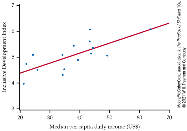
Figure 2.16 Scatterplot of the Inclusive Development Index (IDI) and median per capita daily income for 15 countries that rank high on financial development, Example 2.22.
Fitting a line to data
When a scatterplot displays a linear pattern, we can describe the overall pattern by drawing a regression line through the points. Of course, no straight line passes exactly through all the points. Fitting a line to data means drawing a line that comes as close as possible to the points. The equation of a line fitted to the data gives a concise description of the relationship between the response variable y and the explanatory variable x. It is the numerical summary that supports the scatterplot—our graphical summary.
In practice, we will use software to obtain values of
Example 2.23 Regression line for IDI.
![]()
Any straight line describing the relationship between IDI and MI has the form
In Figure 2.16 we have drawn the regression line with the equation
To make the plot, we chose two values of MI within the range of the
data and evaluated the value of IDI using the regression equation.
In this case, for example, we chose
and
We plotted these two points,
Figure 2.16 shows that the
regression line fits the data reasonably well. The slope
Check-in
-
2.13 A regression line. A regression equation is
What is the slope of the regression line?
What is the intercept of the regression line?
-
Use the regression equation to find the values of y for
-
Plot the regression line for values of x between 0 and 60.
-
2.14 Plot a line. Make a plot of the data in Example 2.22 and plot the line
on your sketch. Explain why this line does not give a good fit to the data.

Prediction
We can use a regression line to make a prediction of the response y for a specific value of the explanatory variable x. We can interpret the prediction as the average value of y corresponding to a collection of cases at the particular value of x or as our best guess of the value of y for a case with the particular value of x.
Example 2.24 Visualize the prediction for IDI.
![]()
Based on the linear pattern, we want to predict IDI for a country
whose MI is $40. To use the fitted line to predict IDI, go “up and
over” on the graph in
Figure 2.17. From
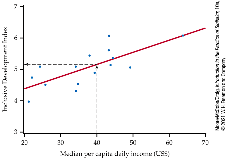
Figure 2.17 The dashed line indicates how to use the regression line to predict the IDI for a country with a median per capita daily income of $40, Example 2.24.
If we have the equation of the line, it is faster and more accurate
to substitute
The degree of uncertainty of predictions from a regression line depends on how much scatter about the line the data show. In Figure 2.17, IDI for values of MI around 40 show a spread of 0.5 unit.
Check-in
-
2.15 Predict the IDI. Use the regression equation in Example 2.20 to predict the IDI for a country whose MI is $35.
The least-squares regression line
![]()
Different people might draw different lines by eye on a scatterplot. This is especially true when the points are widely scattered. We need a way to draw a regression line that doesn’t depend on our guess as to where the line should go. We will use the least-squares idea to select the best regression line. To get started, we’ll think about the distance between an observed value of the response variable (a data point on a scatterplot) and the corresponding value for that case on the regression line predicted by an equation.
Let’s look at the World Economic Forum data for Canada. From
Example 2.22 (page 99), we see that
For Canada, the distance between the observed value of IDI and the predicted value of IDI is
Note that this distance is negative. Distances are negative if the observed response lies below the line and positive if the response lies above the line.
Check-in
-
2.16 Find a distance. Use the regression line in Example 2.23 to estimate the IDI for Italy. What is the distance between the observed IDI for Italy and this predicted value?
-
2.17 Positive and negative distances. Examine Figure 2.16 carefully. How many of the distances are positive? How many are negative?
We are now ready to describe the least-squares idea and the least-squares line. No line will pass exactly through all the points. Even so, we want the distances of the data points from the line to be as small as possible.
Example 2.25 The least-squares idea.
Figure 2.18 illustrates the idea. This plot shows some of the data, along with a regression line. The distances of the data points from the line appear as vertical dashed line segments.
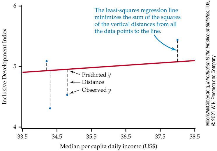
Figure 2.18 The least-squares idea, Example 2.25. For each observation, find the vertical distance of each point from a regression line. The least-squares regression line makes the sum of the squares of these distances as small as possible.
One reason for the popularity of the least-squares regression line is that the problem of finding the line has a simple solution. We can give the recipe for the least-squares line in terms of the means and standard deviations of the two variables and their correlation.
We write
Example 2.26 The equation for predicting IDI.
![]()
The line in Figure 2.16 is, in fact, the least-squares regression line for predicting the IDI from the MI. Software gives the equation of this line as
It is estimated using data from 15 countries that ranked high on the IDI.
Example 2.27 Check the calculation of the line.
![]()
We can check the calculation of the least-squares regression line given in Example 2.26 by using the means and standard deviations for x (MI) and y (IDI) as well as the correlation between these two variables. Here are the pieces we need:
and
The slope is
and the intercept is
The equation of the least-squares line is indeed
![]() When doing calculations like this by hand, you may need to carry
extra decimal places in the preliminary calculations to get accurate
values of the slope and intercept.
In practice, you don’t need to calculate the means, standard
deviations, and correlation first. Statistical software or your
calculator will give the slope
When doing calculations like this by hand, you may need to carry
extra decimal places in the preliminary calculations to get accurate
values of the slope and intercept.
In practice, you don’t need to calculate the means, standard
deviations, and correlation first. Statistical software or your
calculator will give the slope
![]() Be careful, though: different software packages and calculators
label the slope and intercept differently in their output,
so remember that the slope is the value that multiplies x in
the equation.
Be careful, though: different software packages and calculators
label the slope and intercept differently in their output,
so remember that the slope is the value that multiplies x in
the equation.
Example 2.28 Regression using software.
![]()
Figure 2.19 displays regression output for the IDI data from three statistical software packages. You can find the slope and intercept of the least-squares line, calculated to more decimal places than we need, in each output. The software also provides information that we do not yet need, including some that we did not include in Figure 2.19.
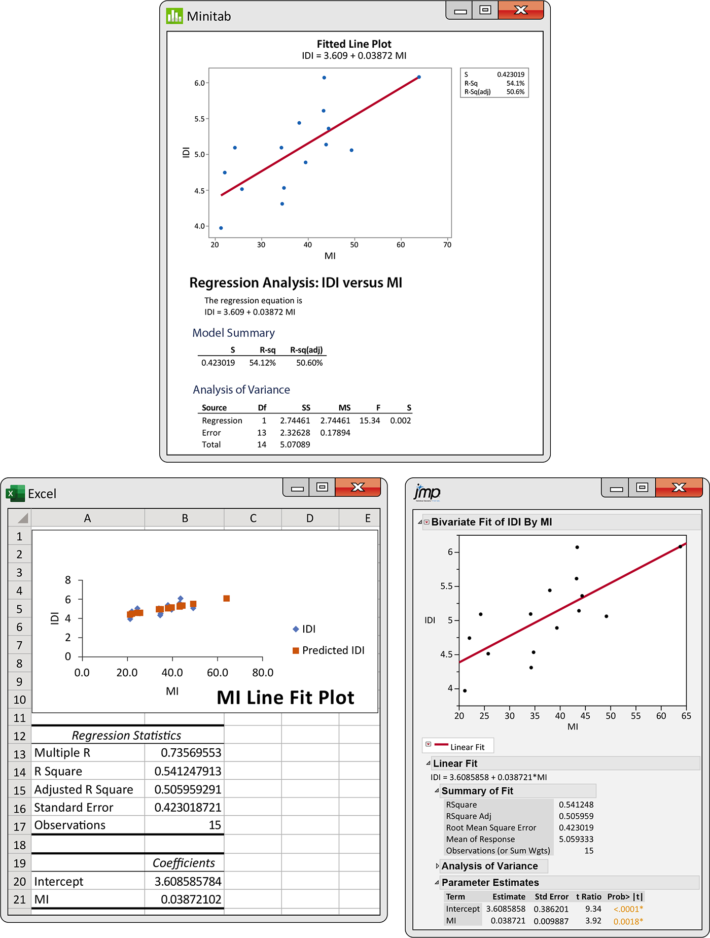
Figure 2.19 Selected least-squares regression outputs for the world financial markets data, Example 2.28. Other software produces similar output.
Part of the art of using software is to ignore the extra information that is almost always present. Look for the results that you need. Once you understand a statistical method, you can read output from almost any software.
Check-in
-
2.18 Predicted values for MI and IDI. Refer to the World Economic Forum data in Example 2.22.
-
Use software to compute the coefficients of the regression equation. Indicate where to find the slope and the intercept on the output and report these values.
-
Make a scatterplot of the data with the least-squares line.
-
For Japan, the IDI is 4.51 and the MI is $34.8. Find the predicted value of IDI for Japan.
-
Find the difference between the actual value and the predicted value for Japan.
-
Facts about least-squares regression
The use of regression to describe the relationship between a response variable and an explanatory variable is one of the most commonly encountered statistical methods, and least-squares is the most commonly used technique for fitting a regression line to data. Here are some facts about least-squares regression lines.
Fact 1. There is a close connection between correlation and the slope of the least-squares line. The slope is
This equation says that along the regression line,
a change of 1 standard deviation in x corresponds to a change of r
standard deviations in y. When the variables are perfectly correlated
Fact 2. The least-squares regression line always passes through the
point
Fact 3. The distinction between explanatory and response variables is essential in regression. Least-squares regression looks at the distances of the data points from the line only in the y direction. If we reverse the roles of the two variables, we get a different least-squares regression line.
Example 2.29 World Economic Forum.
![]()
Figure 2.20 is a scatterplot of the World Economic Forum data described in Example 2.22 (page 99). There is a moderate positive linear relationship between Inclusive Development Index (IDI) and median per capita income (MI).
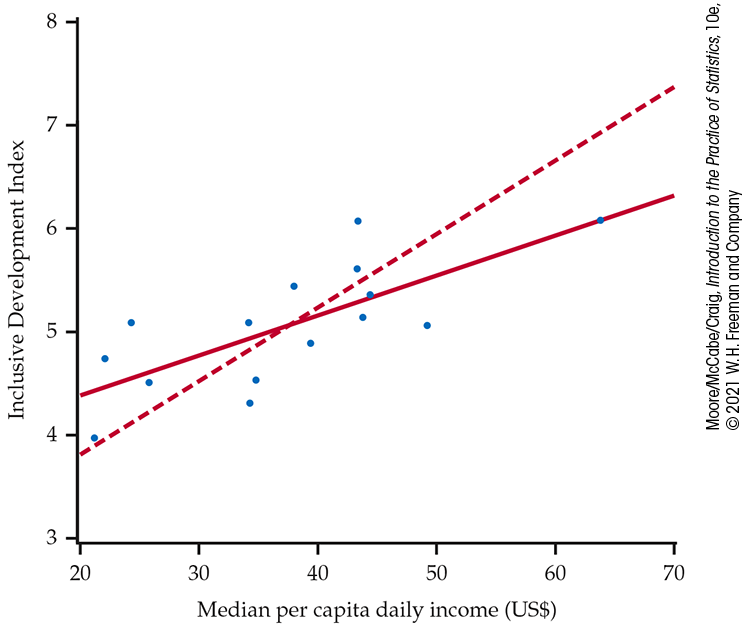
Figure 2.20 Scatterplot of Inclusive Development Index (IDI) versus median per capita income (MI). The two lines are the least-squares regression lines: using MI to predict IDI (solid) and using IDI to predict MI (dashed), Example 2.29.
The two lines on the plot are the two least-squares regression lines. The regression line for using MI to predict IDI is solid, while the regression line for using IDI to predict MI is dashed. The two regressions give different lines. In the regression setting, you must choose one variable to be the explanatory variable.
Correlation and regression
Even though the correlation r ignores the distinction between explanatory and response variables, there is a close connection between correlation and regression. We saw that the slope of the least-squares line involves r. Another connection between correlation and regression is even more important. In fact, the numerical value of r as a measure of the strength of a linear relationship is best interpreted by thinking about regression.
Example 2.30 Using
r 2
The correlation between the MI and the IDI in
Example 2.22 (page 99) is
When you see a correlation, square it to get a better feel for the
strength of the association. Perfect correlation
Check-in
-
2.19 What fraction of the variation is explained? Consider the following correlations:
Interpretation of
r 2
Here is an explanation of why the square of the correlation
r describes the variation explained by the least-squares
regression. Think about trying to predict a new value of y.
With no other information than our sample of values of y, a
reasonable choice is
Now consider how your prediction would change if you had an
explanatory variable. If we use the regression equation for the
prediction, we use the equation
Let’s compare our two choices for predicting y. With the
explanatory variable x, we use
The numerator represents the variation in y that is explained
by x, and the denominator represents the total variation in
y. In
Chapter 11, where
Section 2.4 SUMMARY
-
A regression line is a straight line that describes how a response variable y changes as an explanatory variable x changes.
-
The most common method of fitting a line to a scatterplot is least squares. The least-squares regression line is the straight line
-
You can use a regression line to predict the value of y for any value of x by substituting this x into the equation of the line.
-
The slope
-
The intercept
-
The least-squares regression line of y on x is the line with slope
-
Correlation and regression are closely connected. The correlation r is the slope of the least-squares regression line when we measure both x and y in standardized units. The square of the correlation
Section 2.4 EXERCISES
-
2.49 Blueberries and anthocyanins. In Exercise 2.8 (page 88), you examined the relationship between Antho3 and Antho4, two anthocyanins found in blueberries. In Exercise 2.30 (page 96), you found the correlation between these two variables.

-
Find the equation of the least-squares regression line for predicting Antho3 from Antho4.
-
Make a scatterplot of the data with the fitted line.
-
How well does the line fit the data? Explain your answer.
-
Use the line to predict the value of Antho3 when Antho4 is equal to 1.7.
-
-
2.50 Fuel consumption. In Exercise 2.11 (page 88), you examined the relationship between

-
Find the equation of the least-squares regression line for predicting
-
Make a scatterplot of the data with the fitted line.
-
How well does the line fit the data? Explain your answer.
-
Use the line to predict the value of
-
-
2.51 Fuel consumption for different types of vehicles. In Exercise 2.13 (page 89), you examined the relationship between

-
Find the least-squares regression equation for predicting
-
Make a scatterplot of the data with the fitted line.
-
Based on what you learned from Exercise 2.13, do you think that a single least-squares regression line provides a good fit for all four types of vehicles? Explain your answer.
-
-
2.52 Bone strength. Exercise 2.14 (page 89), gives the bone strengths of the dominant and the nondominant arms for 15 men who were controls in a study.

-
Plot the data. Use the bone strength in the nondominant arm as the explanatory variable and bone strength in the dominant arm as the response variable.
-
The least-squares regression line for these data is
Add this line to your plot.
-
Use the scatterplot (a graphical summary) with the least-squares line (a graphical display of a numerical summary) to write a short paragraph describing this relationship.
-
-
2.53 Bone strength for baseball players. Refer to the previous exercise. Similar data for baseball players are given in Exercise 2.15 (page 89). Here is the equation of the least-squares line for the baseball players:
Answer parts (a) and (c) of the previous exercise for these data.
-
2.54 Predict the bone strength. Refer to Exercise 2.52. A young male who is not a baseball player has a bone strength of 16.0 Nm/1000 in his nondominant arm. Predict the bone strength in the dominant arm for this person.
-
2.55 Predict the bone strength for a baseball player. Refer to Exercise 2.53. A young male who is a baseball player has a bone strength of 16.0 Nm/1000 in his nondominant arm. Predict the bone strength in the dominant arm for this person.
-
2.56 Compare the predictions. Refer to the two previous exercises. You have predicted two dominant-arm bone strengths: one for a baseball player and one for a person who is not a baseball player. The nondominant bone strengths are both 16.0 Nm/1000.
-
Compare the two predictions by computing the difference in means, baseball player minus control.
-
Explain how the difference in the two predictions is an estimate of the effect of baseball throwing exercise on the strength of arm bones.
-
For nondominant arm strengths of 12 Nm/1000 and 20 Nm/1000, repeat your predictions and take the differences. Make a table of the results of all three calculations (for 12, 16, and 20 Nm/1000).
-
Write a short summary of the results of your calculations for the three different nondominant-arm strengths. Be sure to include an explanation of why the differences are not the same for the three nondominant-arm strengths.
-
-
2.57 Least-squares regression for radioactive decay. Refer to Exercise 2.22 (page 90) for the data on radioactive decay of barium-137m. Here are the data:

Time 1 3 5 7 Count 578 317 203 118 -
Using the least-squares regression equation
find the predicted values for the counts.
-
Compute the differences, observed count minus predicted count. How many of these are positive? How many are negative?
-
Square and sum the differences that you found in part (b).
-
Repeat the calculations that you performed in parts (a), (b), and (c) using the equation
-
In a short paragraph, explain the least-squares idea using the calculations that you performed in this exercise.
-
-
2.58 Least-squares regression for the log counts. Refer to Exercise 2.23 (page 90), where you analyzed the radioactive decay of barium-137m data using log counts. Here are the data:
Time 1 3 5 7 Log count 6.35957 5.75890 5.31321 4.77068 -
Using the least-squares regression equation
find the predicted values for the log counts.
-
Compute the differences, observed count minus predicted count. How many of these are positive? How many are negative?
-
Square and sum the differences that you found in part (b).
-
Repeat the calculations that you performed in parts (a) to (c) using the equation
-
In a short paragraph, explain the least-squares idea using the calculations that you performed in this exercise.
-
-
2.59 College students by state. How well does the population of a state predict the number of undergraduates? The National Center for Education Statistics collects data for each of the 50 U.S. states that we can use to address this question.18

-
Make a scatterplot with population on the x axis and number of undergraduates on the y axis.
-
Describe the form, direction, and strength of the relationship. Are there any outliers?
-
For the number of undergraduates, the mean is 302,136 and the standard deviation is 358,460, and for population, the mean is 5,955,551 and the standard deviation is 6,620,733. The correlation between the number of undergraduates and the population is 0.98367. Use this information to find the least-squares regression line. Show your work.
Add the least-squares line to your scatterplot.
-
-
2.60 College students by state without the four largest states. Refer to the previous exercise. Let’s eliminate the four largest states, which have populations greater than 15 million. Here are the numerical summaries: for number of undergraduate college students, the mean is 220,134 and the standard deviation is 165,270; for population, the mean is 4,367,448 and the standard deviation is 3,310,957. The correlation between the number of undergraduate college students and the population is 0.97081. Use this information to find the least-squares regression line. Show your work.

-
2.61 Make predictions and compare. Refer to the two previous exercises. Consider a state with a population of 4 million. (This value is approximately the median population for the 50 states.)
-
Using the least-squares regression equation for all 50 states, find the predicted number of undergraduate college students.
-
Do the same using the least-squares regression equation for the 46 states with populations less than 15 million.
-
Compare the predictions that you made in parts (a) and (b). Write a short summary of your results and conclusions. Pay particular attention to the effect of including the four states with the largest populations in the prediction equation for a median-sized state.
-
-
2.62 College students by state. Refer to Exercise 2.59, where you examined the relationship between the number of undergraduate college students and the populations for the 50 states. Figure 2.21 gives the output from a software package for the regression. Use this output to answer the following questions.
-
What is the equation of the least-squares regression line?
-
What is the value of
-
Interpret the value of
-
Does the software output tell you that the relationship is linear and not, for example, curved? Explain your answer.
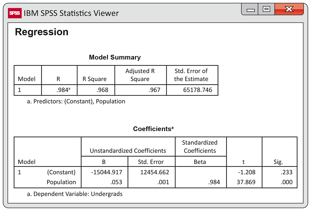
Figure 2.21 SPSS output for predicting number of undergraduate college students, using the population for the 50 U.S. states, Exercise 2.62.
-
-
2.63 College students by state without the four largest states. Refer to Exercise 2.60, where you eliminated the four largest states that have populations greater than 15 million. Figure 2.22 gives software output for these data. Answer the questions in the previous exercise for the data set with the 46 states.
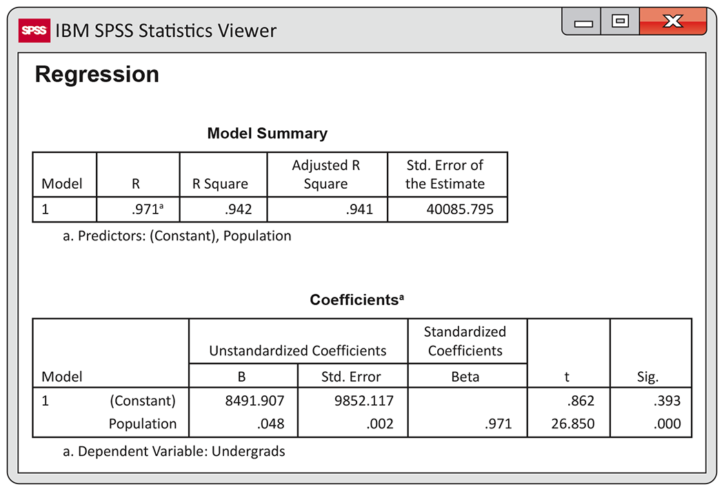
Figure 2.22 SPSS output for predicting number of undergraduate college students using population, with the four largest states deleted, Exercise 2.63.
-
2.64 Data generated by software. The following 20 observations on Y and X were generated by a computer program:

X Y X Y 23.07 35.49 18.85 28.17 19.88 30.38 19.96 31.17 18.83 26.13 17.87 27.74 22.09 31.85 20.20 30.01 17.19 26.77 20.65 29.61 20.72 29.00 20.32 31.78 18.10 28.92 21.37 32.93 18.01 26.30 17.31 30.29 18.69 29.49 23.50 28.57 18.05 31.36 22.02 29.80 -
Make a scatterplot and describe the relationship between Y and X.
-
Find the equation of the least-squares regression line and add the line to your plot.
-
What percent of the variability in Y is explained by X?
-
Summarize your analysis of these data in a short paragraph.
-
-
2.65 Add an outlier. Refer to Exercise 2.64. Add an additional observation with

-
2.66 Add a different outlier. Refer to the previous two exercises. Add an additional observation with

-
Repeat the analysis that you performed in Exercise 2.64 and summarize your results, paying particular attention to the effect of this outlier.
-
In this exercise and in the previous one, you added an outlier to the original data set and reanalyzed the data. Write a short summary of the changes in correlations that can result from different kinds of outliers.
-
-
2.67 Alcohol and calories in beer. Figure 2.12 (page 90) gives a scatterplot of calories versus percent alcohol in 160 brands of domestic beer.

-
Find the equation of the least-squares regression line for these data.
-
Find the value of
-
Write a short report on the relationship between calories and percent alcohol in beer. Include graphical and numerical summaries for each variable separately as well as graphical and numerical summaries for the relationship in your report.
-
-
2.68 Alcohol and calories in beer revisited. Refer to the previous exercise. The data that you used includes an outlier.
-
Remove the outlier and answer parts (a), (b), and (c) for the new set of data.
-
Write a short paragraph about the possible effects of outliers on a least-squares regression line and the value of
-
-
2.69 Always plot your data! Table 2.1 presents four sets of data prepared by the statistician Frank Anscombe to illustrate the dangers of calculating without first plotting the data.19

-
Without making scatterplots, find the correlation and the least-squares regression line for all four data sets. What do you notice? Use the regression line to predict y for
-
Make a scatterplot for each of the data sets and add the regression line to each plot.
-
In which of the four cases would you be willing to use the regression line to describe the dependence of y on x? Explain your answer in each case.
Table 2.1 Four data sets for exploring correlation and regression
Data Set A x 10 8 13 9 11 14 6 4 12 7 5 y 8.04 6.95 7.58 8.81 8.33 9.96 7.24 4.26 10.84 4.82 5.68 Data Set B x 10 8 13 9 11 14 6 4 12 7 5 y 9.14 8.14 8.74 8.77 9.26 8.10 6.13 3.10 9.13 7.26 4.74 Data Set C x 10 8 13 9 11 14 6 4 12 7 5 y 7.46 6.77 12.74 7.11 7.81 8.84 6.08 5.39 8.15 6.42 5.73 Data Set D x 8 8 8 8 8 8 8 8 8 8 19 y 6.58 5.76 7.71 8.84 8.47 7.04 5.25 5.56 7.91 6.89 12.50 -
-
2.70 Progress in math scores. Every few years, the National Assessment of Educational Progress asks a national sample of eighth-graders to perform the same math tasks. The goal is to get an honest picture of progress in math. Here are a few national mean scores, on a scale of 0 to 500:20

Year 1990 2000 2009 2017 2019 Score 263 273 283 283 282 -
Make a time plot of the mean scores. This is just a scatterplot of score against year. There is a slow linear increasing trend.
-
Find the regression line of mean score on time step-by-step. First calculate the mean and standard deviation of each variable and their correlation. Then find the equation of the least-squares line from these. Draw the line on your scatterplot. What percent of the year-to-year variation in scores is explained by the linear trend?
Now use software to verify your regression line.
-
Does the regression line give a good fit to the data? Explain your answer.
-
-
2.71 The regression equation. The equation of a least-squares regression line is
-
What is the value of y for
-
If x increases by one unit, what is the corresponding change in y?
What is the intercept for this equation?
-
-
2.72 Metabolic rate and lean body mass. Compute the mean and the standard deviation of the metabolic rates and lean body masses in Exercise 2.27 (page 91) and the correlation between these two variables. Use these values to find the slope of the regression line of metabolic rate on lean body mass. Also find the slope of the regression line of lean body mass on metabolic rate. What are the units for each of the two slopes?

-
 2.73 Use an applet for progress in math scores.
Go to the Two-Variable Statistical Calculator applet.
Enter the data for the progress in math scores from
Exercise 2.70. Using
only the results provided by the applet, write a short report
summarizing the analysis of these data.
2.73 Use an applet for progress in math scores.
Go to the Two-Variable Statistical Calculator applet.
Enter the data for the progress in math scores from
Exercise 2.70. Using
only the results provided by the applet, write a short report
summarizing the analysis of these data.
-
 2.74 A property of the least-squares regression line.
Use the equation for the least-squares regression line to show
that this line always passes through the point
2.74 A property of the least-squares regression line.
Use the equation for the least-squares regression line to show
that this line always passes through the point
-
2.75 Class attendance and grades. A study of class attendance and grades among first-year students at a state university showed that, in general, students who missed a higher percent of their classes earned lower grades. Class attendance explained 25% of the variation in grade index among the students. What is the numerical value of the correlation between percent of classes attended and grade index?