4.5 General Probability Rules
Our study of probability has concentrated on random variables and their distributions. Now we return to the rules that govern any assignment of probabilities. The purpose of learning more rules of probability is to be able to develop and work with probability models for more complex random phenomena.
We have already met and used the following five rules.
Let’s now consider more general addition and multiplication rules.
General addition rules
Probability has the property that if A and B are
disjoint events, then
Suppose now that we have several events—say, A, B, and C—that are disjoint in pairs. That is, no two can occur simultaneously. The Venn diagram in Figure 4.15 illustrates three disjoint events.
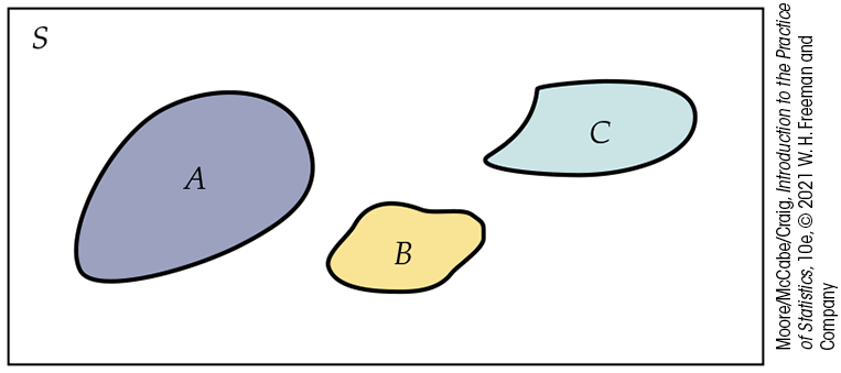
Figure 4.15 The
addition rule for disjoint events:
The addition rule for two disjoint events extends to the following rule.
Example 4.53 Probabilities as areas.
Generate a random number X between 0 and 1. What is the probability that the first digit after the decimal point will be a 3, 6, or 9? The random number X is a continuous random variable whose density curve has constant height 1 between 0 and 1 and is 0 elsewhere. These events are
Figure 4.16 illustrates the probabilities of these events as areas under the density curve. Let’s examine the first four probability rules with this example.
-
Rule 1:
-
Rule 2:
-
Rule 3: If A and B are disjoint events, then
-
Rule 4:
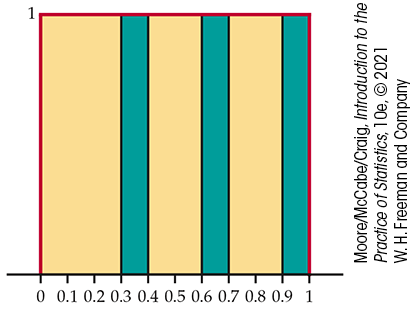
Figure 4.16 The probability that the first digit after the decimal point of a random number is a 3, a 6, or a 9 is the sum of the probabilities of the three disjoint events shown, Example 4.53.
Check-in
-
4.21 Probability that you roll an even number less than 5. If you roll a die, the probability of each of the six possible outcomes (1, 2, 3, 4, 5, 6) is 1/6. What is the probability that you roll an even number less than 5? What probability rules did you use to find your answer.
If events A and B are not disjoint, they can occur simultaneously. This introduces a new combination of events called the union. The probability of their union is then less than the sum of their probabilities.
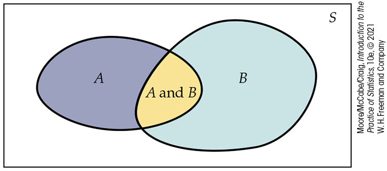
Figure 4.17 The union
of two events that are not disjoint. The general addition rule
says that
For two events A and B, the union is the event {A or B} that A or B or both occur. From the addition rule for two disjoint events, we can obtain rules for more general unions.
As Figure 4.17 suggests, the outcomes common to both are counted twice when we add probabilities, so we must subtract this probability once. Here is the addition rule for the union of any two events, disjoint or not.
If A and B are disjoint, the event {A and
B} that both occur has no outcomes in it. This
empty event is the complement of the sample space S and
must have probability 0. So, our probability Rule 3 is a special case
of the general addition rule, where A and B are disjoint and,
therefore,
Example 4.54 Adequate sleep and exercise.

Suppose that 40% of adults get enough sleep and 46% exercise regularly. What is the probability that an adult either gets enough sleep or exercises regularly? To find this probability, we also need to know the percent who get enough sleep and exercise. Let’s assume this is 24%.
We will use the notation of the general addition rule for unions of
two events. Let A be the event that an adult gets enough
sleep, and let B be the event that a person exercises
regularly. We are given that
The probability that an adult either gets enough sleep or exercises regularly is 0.62, or 62%.
Check-in
-
4.22 Probability that your roll is odd or less than 3. If you roll a die, the probability of each of the six possible outcomes (1, 2, 3, 4, 5, 6) is 1/6. What is the probability that your roll is odd or less than 3?
Venn diagrams provide great help in finding probabilities for unions because you can just think of adding and subtracting areas. Figure 4.18 shows some events and their probabilities for Example 4.54. What is the probability that an adult gets adequate sleep and does not exercise?
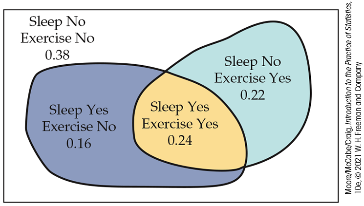
Figure 4.18 Venn diagram and probabilities, Example 4.54.
The Venn diagram shows that the probability that an adult gets
adequate sleep minus the probability that an adult gets adequate sleep
and exercises regularly is
Conditional probability
Now let’s revisit the multiplication rule that so far has focused on independent events. The probability we assign to an event can change if we know that some other event has occurred. This idea is the key to many applications of probability.
Example 4.55 Probability of being dealt a heart.
Doyle is a professional poker player and is about to get the last of his five cards for his hand. What is the probability that the card dealt to Doyle is a heart? There are 52 cards in the deck. Because the deck was carefully shuffled, the next card dealt is equally likely to be any of the 52 cards in the deck. Because 13 of the 52 cards are hearts,
This calculation assumes that Doyle knows nothing about his 4 cards
already dealt. Suppose that he looked at those 4 and knows they are
all hearts. He knows nothing about the other 48 cards except that
exactly 9
Knowing that there are 4 hearts among the 4 cards changes the probability that the next card dealt is a heart.
The new notation
Check-in
-
4.23 The probability of a heart. Refer to Example 4.55. Suppose that two of the four cards in Doyle’s hand are hearts. What is the probability that the next card dealt to him will be a heart?
The multiplication rule is just common sense made formal.
Example 4.56 Downloading music from the Internet.
Suppose that 30% of Internet users download music files, and 70% of downloaders say they don’t care if the music is copyrighted. The percent of Internet users who download music (event A) and don’t care about copyright (event B) is 70% of the 30% who download, or
The multiplication rule expresses this as
Here is another example that uses conditional probability.
Example 4.57 Probability of a favorable draw.
Doyle is still at the poker table. At the moment, he has 2 cards,
and they are both hearts. He has seen 24 cards, and none of other
players have any hearts. What is the chance that the next 3 cards he
draws will be hearts? The full deck of 52 cards contains 13 hearts.
Therefore, 11 of the unseen cards are hearts. There are 28
Doyle finds these probabilities by counting cards. The probability that the first card drawn is a heart is 11/28 because 11 of the 28 unseen cards are hearts. If the first card is a heart, that leaves 10 hearts among the 27 remaining cards. So the conditional probability of another heart is 10/27. The multiplication rule now says that
We again apply the multiplication rule for the third card. The probability that the next 3 draws are hearts is equal to the probability that the first 2 draws are hearts times the probability that the third card is a heart given that the first 2 draws are hearts. This probability is
It is very unlikely that Doyle’s next 3 cards will be hearts, even though his hearts are the only ones that he has seen.
Check-in
-
4.24 The probability that the next two cards are hearts. In the setting of Example 4.55, suppose that Doyle’s third card is a heart, so that he now has three hearts, and that none of the five additional cards that he sees are hearts. What is the probability that the next two cards dealt to Doyle will be hearts?
If P(A) and P(A and B) are given, we can
rearrange the multiplication rule to produce a definition of
the conditional probability
![]() Be sure to keep in mind the distinct roles in
Be sure to keep in mind the distinct roles in
Example 4.58 College students.
Here is the distribution of U.S. college students classified by age and full-time or part-time status:
| Age (years) | Full-time | Part-time |
|---|---|---|
| 15 to 19 | 0.21 | 0.02 |
| 20 to 24 | 0.32 | 0.07 |
| 25 to 34 | 0.10 | 0.10 |
| 30 and over | 0.05 | 0.13 |
Note that the sum of the probabilities is one. Let’s compute the probability that a student is aged 20 to 24, given that the student is full-time. We know that the probability that a student is full-time and aged 20 to 24 is 0.32 from the table of probabilities. But what we want here is a conditional probability, given that a student is full-time. Rather than ask about age among all students, we restrict our attention to the subpopulation of students who are full-time. Let
Our formula is
We read
We are now ready to complete the calculation of the conditional probability:
The probability that a student is 20 to 24 years of age, given that the student is full-time, is 0.47.
Here is another way to give the information in the last sentence of this example: 47% of full-time college students are 20 to 24 years old. Which way do you prefer?
Check-in
-
4.25 What rule did we use? In Example 4.58, we calculated P(B). What rule did we use for this calculation? Explain why the rule applies in this setting.
-
4.26 Find the conditional probability. Refer to Example 4.58. What is the probability that a student is part-time, given that the student is 25 to 34 years old? Explain in your own words the difference between this calculation and the one that we did in Example 4.58.
General multiplication rules
The definition of conditional probability reminds us that, in principle, all probabilities—including conditional probabilities—can be found from the assignment of probabilities to events that describe random phenomena. More often, however, conditional probabilities are part of the information given to us in a probability model, and the multiplication rule is used to compute P(A and B). This rule extends to more than two events.
The union of a collection of events is the event that any of them occur. Here is the corresponding term for the event that all of them occur.
To extend the multiplication rule to the probability that all of several events occur, the key is to condition each event on the occurrence of all the preceding events. For example, the intersection of three events A, B, and C, as in Example 4.57, has probability
Here is another example.
Example 4.59 High school athletes and professional careers.
Only 5% of male high school basketball, baseball, and football players go on to play at the college level. Of these, only 1.7% enter major league professional sports. About 40% of the athletes who compete in college and then reach the pros have a career of more than three years. Define these events:
What is the probability that a high school athlete competes in college and then goes on to have a pro career of more than three years? We know that
Therefore, the probability we want is
Only about 3 of every 10,000 high school athletes can expect to compete in college and have a professional career of more than three years. High school students would be wise to concentrate on studies rather than on unrealistic hopes of fortune from pro sports.
Tree diagrams
Probability problems often require us to combine several of the basic rules into a more elaborate calculation. Here is an example that illustrates how to solve problems that have several stages.
Example 4.60 Online chat rooms.
Online chat rooms are dominated by the young. Teens are the biggest
users. If we look only at adult Internet users (aged 18 and over),
47% of the 18 to 29 age group chat, as do 21% of the 30 to 49 age
group and just 7% of those 50 and over. To learn what percent of all
Internet users participate in chat, we also need the age breakdown
of users. Here it is: 29% of adult Internet users are 18 to 29 years
old (event
What is the probability that a randomly chosen adult user of the Internet participates in chat rooms (event C)? To find out, use the tree diagram in Figure 4.19 to organize your thinking. Each segment in the tree is one stage of the problem. Each complete branch shows a path through the two stages. The probability written on each segment is the conditional probability of an Internet user following that segment, given that he or she has reached the node from which it branches.
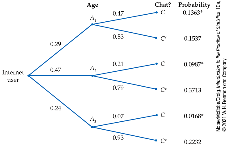
Figure 4.19 Tree diagram, Example 4.60. The probability P(C) is the sum of the three probabilities of the three branches marked with asterisks (*).
Starting at the left, an Internet user falls into one of the three age groups. The probabilities of these groups
mark the leftmost branches in the tree. Conditional on being 18 to
29 years old, the probability of participating in chat is
These conditional probabilities mark the paths branching out from
the
There are three disjoint paths to C, one for each age group. By the addition rule, P(C) is the sum of their probabilities. The probability of reaching C through the 18 to 29 age group is
Follow the paths to C through the other two age groups. The probabilities of these paths are
The final result is
About 25% of all adult Internet users take part in chat rooms.
It takes longer to explain a tree diagram than it does to use it. Once you have understood a problem well enough to draw the tree, the rest is easy. Tree diagrams combine the addition and multiplication rules. The multiplication rule says that the probability of reaching the end of any complete branch is the product of the probabilities written on its segments. The probability of any outcome, such as the event C that an adult Internet user takes part in chat rooms, is then found by adding the probabilities of all branches that are part of that event.
Check-in
-
4.27 Draw a tree diagram. Refer to Doyle’s chances of five hearts in Example 4.57 (page 257). Draw a tree diagram to describe the outcomes for the three cards that he will be dealt. At the first stage, his draw can be a heart or a nonheart. At the second and third stages, he has the same possible outcomes, but the probabilities are different.
Bayes’s rule
There is another kind of probability question that we might ask in the context of thinking about online chat. What percent of adult chat room participants are aged 18 to 29?
Example 4.61 Conditional versus unconditional probabilities.
In the notation of
Example 4.60, this is the conditional probability
More than half of adult chat room participants are between 18 and 29 years old. Compare this conditional probability with the original information (unconditional) that 29% of adult Internet users are between 18 and 29 years old. Knowing that a person chats increases the probability that he or she is young.
We know the probabilities
In
Example 4.61, we calculated the “reverse” conditional probability
The numerator in
Bayes’s
rule
is always one of the terms in the sum that makes up the denominator.
The rule is named after Thomas Bayes, who wrestled with arguing from
outcomes like C back to the
Example 4.62 Use Bayes’s rule.
Let’s use Bayes’s rule to compute the value of
We then apply the Bayes’s rule formula
Independence again
The conditional probability
This definition makes precise the informal description of
independence given in
Section 4.1
(page 207). We now
see that the multiplication rule for independent events,
Example 4.63 Are the events independent?
Suppose
Since
Example 4.64 Dependent events.
Suppose
Since
Section 4.5 SUMMARY
-
The complement
-
The conditional probability
when
-
The essential general rules of elementary probability are
-
Legitimate values:
-
Total probability 1:
-
Complement rule:
-
Addition rule:
-
Multiplication rule:
-
-
If A and B are disjoint, then
-
A and B are independent when
-
In problems with several stages, draw a tree diagram to organize use of the multiplication and addition rules.
Section 4.5 EXERCISES
-
4.78 Find and explain some probabilities.
-
Suppose
-
Explain in your own words the meaning of the rule
-
Consider an event A. What is the name for the event that A does not occur? If
-
Suppose that A and B are independent and that
-
Suppose
-
-
4.79 Probability rules.
-
Explain why a probability cannot be less than zero or greater than one.
-
What is the probability of the event that A or
-
If A and B are disjoint, what is the probability of A or B?
-
What is the probability of the complement of A in terms of the probability of A?
-
If A and B are independent, what is the probability of A and B in terms of the probability of A and the probability of B?
-
-
4.80 Why not? Suppose that
-
4.81 Unions. Assume that
-
4.82 The complement. Refer to the previous exercise. Find the probability of the complement of the union of A, B, and C.
-
4.83 Find the probability. Suppose that the probability that A occurs is 0.6 and the probability that A and B occur is 0.3. Find the probability that B occurs, given that A occurs and illustrate your calculations using a Venn diagram.
-
4.84 Is the calcium intake adequate? In the population of young children eligible to participate in a study of whether or not their calcium intake is adequate, 52% are 5 to 10 years of age and 48% are 11 to 13 years of age. For those who are 5 to 10 years of age, 18% have inadequate calcium intake. For those who are 11 to 13 years of age, 57% have inadequate calcium intake.17
-
Use letters to define the events of interest in this exercise.
-
Convert the percents given to probabilities of the events you have defined.
-
Use a tree diagram similar to Figure 4.19 (page 261) to calculate the probability that a randomly selected child from this population has an inadequate intake of calcium.
-
-
4.85 Find a probability. Suppose that
-
4.86 Another probability. Refer to the previous exercise. What is the probability of the event that B occurs and A does not?
-
4.87 Use Bayes’s rule. Refer to Exercise 4.84. Use Bayes’s rule to find the probability that a child from this population who has inadequate intake is 5 to 10 years old.
-
4.88 What’s wrong? In each of the following scenarios, there is something wrong. Describe what is wrong and give a reason for your answer.
-
P(A or B) is always equal to the sum of P(A) and P(B).
-
The probability of an event minus the probability of its complement is always equal to 1.
-
Two events are disjoint if
-
-
4.89 Are the events independent? Refer to Exercises 4.84 and 4.87. Are the age of the child and whether or not the child has adequate calcium intake independent? Calculate the probabilities that you need to answer this question and write a short summary of your conclusion.
-
4.90 Exercise and sleep. Suppose that 46% of adults get enough sleep, 40% get enough exercise, and 27% do both. Find the probabilities of the following events:
Enough sleep and not enough exercise.
Not enough sleep and enough exercise.
Not enough sleep and not enough exercise.
-
For each of parts (a), (b), and (c), state the rule that you used to find your answer.
-
4.91 Venn diagram for exercise and sleep. Refer to the previous exercise. Draw a Venn diagram showing the probabilities for exercise and sleep.
-
4.92 Find a probability for lying to a teacher. Suppose that 46% of high school students would admit to lying at least once to a teacher during the past year and that 28% of students are male and would admit to lying at least once to a teacher during the past year.18 Assume that 44% of the students are male. What is the probability that a randomly selected student is either male or would admit to lying to a teacher during the past year? Be sure to show your work and indicate all the rules that you use to find your answer.
-
4.93 Find another probability for lying to a teacher. Refer to the previous exercise. Suppose that you select a student from the subpopulation of those who would admit to lying to a teacher during the past year. What is the probability that the student is female? Be sure to show your work and indicate all the rules that you use to find your answer.
-
 4.94 Attendance at two-year and four-year colleges.
In a large national population of college students, 59% attend
four-year institutions, and the rest attend two-year
institutions. Males make up 44% of the students in the four-year
institutions and 40% of the students in the two-year
institutions.
4.94 Attendance at two-year and four-year colleges.
In a large national population of college students, 59% attend
four-year institutions, and the rest attend two-year
institutions. Males make up 44% of the students in the four-year
institutions and 40% of the students in the two-year
institutions.
-
Find the four probabilities for each combination of sex and type of institution in the following table. Be sure that your probabilities sum to 1.
Male Female Four-year institution Two-year institution - Consider randomly selecting a female student from this population. What is the probability that she attends a four-year institution?
-
-
4.95 Draw a tree diagram. Refer to the previous exercise. Draw a tree diagram to illustrate the probabilities in a situation where you first identify the type of institution attended and then identify the gender of the student.
-
4.96 Draw a different tree diagram for the same setting. Refer to the previous two exercises. Draw a tree diagram to illustrate the probabilities in a situation where you first identify the gender of the student and then identify the type of institution attended. Explain why the probabilities in this tree diagram are different from those that you used in the previous exercise.
-
4.97 Education and income. Call a household prosperous if its income exceeds $100,000. Call the household educated if the householder completed college. Select an American household at random and let A be the event that the selected household is prosperous and B the event that it is educated. According to the Current Population Survey,
-
4.98 Find a conditional probability. In the setting of the previous exercise, what is the conditional probability that a household is prosperous, given that it is educated? Explain why your result shows that events A and B are not independent.
-
4.99 Draw a Venn diagram. Draw a Venn diagram that shows the relation between the events A and B in Exercise 4.97. Indicate each of the following events on your diagram and use the information in Exercise 4.97 to calculate the probability of each event. Finally, describe in words what each event is.
-
{A and B}.
-
{
-
{A and
-
{
-
-
4.100 Sales of cars and light trucks. Motor vehicles sold to individuals are classified as either cars or light trucks (including SUVs) and as either domestic or imported. In a recent year, 72% of vehicles sold were light trucks, 68% were domestic, and 54% were domestic light trucks. Let A be the event that a vehicle is a car and B the event that it is imported. Write each of the following events in set notation and give its probability.
The vehicle is a light truck.
The vehicle is an imported car.
-
4.101 Conditional probabilities and independence.
Using the information in
Exercise 4.100, answer these questions.
-
Given that a vehicle is imported, what is the conditional probability that it is a light truck?
-
Are the events “vehicle is a light truck” and “vehicle is imported” independent? Justify your answer.
-
-
4.102 Job offers. Emily is graduating from college. She has studied biology, chemistry, and computing and hopes to work as a forensic scientist applying her science background to crime investigation. Late one night she thinks about some jobs she has applied for. Let A, B, and C be the events Emily is offered a job by
Emily writes down her personal probabilities for being offered these jobs:
Make a Venn diagram of the events A, B, and C. As in Figure 4.18 (page 256), mark the probabilities of every intersection involving these events and their complements. Use this diagram for Exercises 4.103, 4.104, and 4.105.
-
4.103 Find the probability of at least one offer. What is the probability that Emily is offered at least one of the three jobs?
-
4.104 Find the probability of another event. What is the probability that Emily is offered both the Connecticut and New Jersey jobs but not the federal job?
-
4.105 Find a conditional probability. If Emily is offered the federal job, what is the conditional probability that she is also offered the New Jersey job? If Emily is offered the New Jersey job, what is the conditional probability that she is also offered the federal job?
Genetic counseling. Conditional probabilities and Bayes’s rule are a basis for counseling people who may have genetic defects that can be passed to their children. Exercises 4.106, 4.107, and 4.108 concern genetic counseling settings.
-
4.106 Albinism. People with albinism have little pigment in their skin, hair, and eyes. The gene that governs albinism has two forms (called alleles), which we denote a and A. Each person has a pair of these genes, one inherited from each parent. A child inherits one of each parent’s two alleles independently with probability 0.5. Albinism is a recessive trait, so a person is albino only if the inherited pair is aa.
-
Beth’s parents are not albino, but she has an albino brother. This implies that both of Beth’s parents have type Aa. Why?
-
Which of the types aa, Aa, and AA could a child of Beth’s parents have? What is the probability of each type?
-
Beth is not albino. What are the conditional probabilities for Beth’s possible genetic types, given this fact? (Use the definition of conditional probability.)
-
-
4.107 Find some conditional probabilities. Beth knows the probabilities for her genetic types from part (c) of the previous exercise. She marries Bob, who is albino. Bob’s genetic type must be aa.
-
What is the conditional probability that a child of Beth and Bob is non-albino if Beth has type Aa? What is the conditional probability of a non-albino child if Beth has type AA?
-
Beth and Bob’s first child is non-albino. What is the conditional probability that Beth is a carrier, type Aa?
-
-
4.108 Muscular dystrophy. Muscular dystrophy is an incurable muscle-wasting disease. The most common and serious type, called DMD, is caused by a sex-linked recessive mutation. Specifically, women can be carriers but do not get the disease; a son of a carrier has probability 0.5 of having DMD; a daughter has probability 0.5 of being a carrier. As many as one-third of DMD cases, however, are due to spontaneous mutations in sons of mothers who are not carriers. Toni has one son, who has DMD.
In the absence of other information, the probability is 1/3 that the son is the victim of a spontaneous mutation and 2/3 that Toni is a carrier. There is a screening test called the CK test that is positive with probability 0.7 if a woman is a carrier and with probability 0.1 if she is not. Toni’s CK test is positive. What is the probability that she is a carrier?