2.6 Data Analysis for Two-Way Tables in Chapter 2 Looking at Data

2.6 Data Analysis for Two-Way Tables

When you complete this section, you will be able to:

Identify the row variable, the column variable, and the cells in a two-way table.
Find and interpret the joint distribution in a two-way table.
Find and interpret the marginal distributions in a two-way table.
Use the conditional distributions to describe the relationship displayed in a two-way table.
Find the joint distribution, the marginal distributions, and the conditional distributions in a two-way table from software output.
Interpret examples of Simpson’s paradox.

When we study relationships between two variables, one of the first questions we ask is whether each variable is quantitative or categorical. For two quantitative variables, we use a scatterplot to examine the relationship, and we fit a line to the data if the relationship is approximately linear. If one of the variables is quantitative and the other is categorical, we use the methods in Chapter 1 to describe the distribution of the quantitative variable for each value of the categorical variable. This leaves us with the situation where both variables are categorical. In this section, we discuss methods for studying these relationships.

Some variables—such as sex, race, and occupation—are inherently categorical. Other categorical variables are created by grouping values of a quantitative variable into classes. Published data are often reported in grouped form to save space.

To describe categorical data, we use the counts (frequencies) or percents (relative frequencies) of individuals that fall into various categories. We studied graphical and numerical summaries for a single categorical variable in Chapter 1. There we used pie charts and bar graphs as graphical summaries, and we used counts and percents as numerical summaries. The same tools are useful when we analyze the relationship between a pair of categorical variables.

The two-way table

Data set icon for Vtm.

A key idea in studying relationships between two variables is that both variables must be measured on the same individuals or cases. When both variables are categorical, the raw data are summarized in a two-way table that gives counts of observations for each combination of values of the two categorical variables. Here is an example.

Example 2.40 Is the calcium intake adequate?

Young children need calcium in their diet to support the growth of their bones. The Institute of Medicine provides guidelines for how much calcium should be consumed for people of different ages.²⁴ One study examined whether a sample of children consumed an adequate amount of calcium, based on these guidelines. Because there are different requirements for children aged 5 to 10 years and for children aged 11 to 13 years of age, the children were classified into these two age groups. For each child, his or her calcium intake was classified as meeting or not meeting the requirement. There were 2029 children in the study. Here are the data:²⁵

Two-way table for Met requirement and Age
	Age (years)
Met requirement	5 to 10	11 to 13
No	194	557
Yes	861	417

We see that 194 children aged 5 to 10 did not meet the calcium requirement, and 861 children aged 5 to 10 years met the calcium requirement.

Check-in

2.24 Read the table. Refer to the table in Example 2.40. How many children aged 11 to 13 met the requirement? How many did not?

For the calcium requirement example, we could view Age as an explanatory variable and Met requirement as a response variable. This is why we put Age in the columns (like the x axis in a scatterplot) and Met requirement in the rows (like the y axis in a scatterplot). We call Met requirement the row variable because each horizontal row in the table describes whether or not the requirement was met. Age is the column variable because each vertical column describes one age group. Each combination of values for these two variables is called a cell. For example, the cell corresponding to children who are 5 to 10 years old and who have not met the requirement contains the number 194. This two-way table is called a 2×2 table because there are two rows and two columns.

To describe relationships between two categorical variables, we typically compute different types of percents. This job is made easier if we expand the basic two-way table by adding various totals to the margins, or borders, of the table. We illustrate this idea with our calcium requirement example.

Example 2.41 Add the margins to the table.

The row variable for the table in Example 2.40 is Met requirement, and the column variable is Age. We now expand that table by adding the totals for each row, for each column, and the total number of all the observations. Here is the result:

Two-way table for Met requirement and Age
	Age (years)
Met requirement	5 to 10	11 to 13	Total
No	194	557	751
Yes	861	417	1278
Total	1055	974	2029

With these totals, we can now say more about the study. There were 1055 children aged 5 to 10. The total number of children who did not meet the calcium requirement is 751, and the total number of children in the study is 2029.

Check-in

2.25 Read the margins of the table. How many children aged 11 to 13 were subjects in the calcium requirement study? What is the total number of children who met the calcium requirement?

Be sure that you understand how a two-way table is obtained from the raw data. For the table in Example 2.41, think about a data file with one line per child. There would be 2029 lines or records in this data set. In the two-way table, each individual or case is counted once and only once. As a result, the sum of the counts in the table is the total number of individuals in the data set. caution Most errors in the use of categorical-data methods come from a misunderstanding of how these tables are constructed.

Joint distribution

We are now ready to compute some proportions (percents expressed in decimal form) that help us understand the data in a two-way table. Suppose that we are interested in the children aged 5 to 10 years who do not meet the calcium requirement. The proportion of children in this cell is simply 194 divided by 2029, or 0.0956. We would estimate that 9.56% of children in the population from which this sample was drawn are 5- to 10-year-olds who do not meet the calcium requirement. For each cell, we can compute a proportion by dividing the cell entry by the total sample size. The collection of these proportions is the joint distribution of the two categorical variables.

Example 2.42 The joint distribution.

For the calcium requirement example, the joint distribution of Met requirement and Age is

Joint distribution of Met requirement and Age
	Age (Years)
Met requirement	5 to 10	11 to 13
No	0.0956	0.2745
Yes	0.4243	0.2055

The entries in the table give the proportions of the observations corresponding to the particular row and column. For example, the proportion of the sample who are 5 to 10 years old and do not meet the requirement is 0.0956, or 9.56%. Because this is a distribution, the sum of the proportions should be 1. For this example the sum is 0.9999. The difference is due to roundoff error.

Check-in

2.26 Explain the computation. Explain how the entry for the children aged 5 to 10 who met the calcium requirement in Example 2.42 is computed from the table in Example 2.41.

How might we use the information in the joint distribution for this example? Suppose that we were to develop an outreach unit to increase the consumption of calcium. The distribution suggests that the older children should be targeted if we have to make a choice because of limited funds. Children who are 11 to 13 years old and do not meet the calcium requirement are 27.45% of the total; however, children who are 5 to 10 years old and do not meet the requirement are only 9.56% of the total. For other uses of these data, we may want to calculate different numerical summaries. Let’s now look at the distributions of each variable individually.

Marginal distributions

When we examine the distribution of a single variable in a two-way table, we are looking at a marginal distribution. There are two marginal distributions, one for each categorical variable in the two-way table. They are very easy to compute.

Example 2.43 The marginal distribution of Age.

Look at the table in Example 2.41. The total numbers of children aged 5 to 10 and children aged 11 to 13 are given in the bottom row, labeled “Total.” Our sample has 1055 children aged 5 to 10 and 974 children aged 11 to 13. To find the marginal distribution of age, we simply divide these numbers by the total sample size, 2029. The marginal distribution of Age is

Marginal distribution of Age
	5 to 10	11 to 13
Proportion	0.52	0.48

In the sample, 52% of the children are 5 to 10 years old and 48% of the children are 11 to 13 years old. Note that the proportions sum to 1; there is no roundoff error.

Often, we prefer to use percents rather than proportions. Here is the marginal distribution of age described with percents:

Marginal distribution of Age
	5 to 10	11 to 13
Percent	52%	48%

Which form do you prefer?

The percent of children in each age group is approximately the same. This is interesting because the first category includes six ages (5, 6, 7, 8, 9, and 10), whereas the second includes only three ages (11, 12, and 13). Recall that the age categories were chosen in this way because the Institute of Medicine defined the calcium requirement differently for these age groups.

The other marginal distribution for this example is the distribution of met requirement.

Example 2.44 The marginal distribution of Met requirement.

Here is the marginal distribution of Met requirement, in percents:

Marginal distribution of Met requirement
	No	Yes
Percent	37.01%	62.99%

Check-in

2.27 Explain the marginal distribution. Explain how the marginal distribution of Met requirement given in Example 2.44 is computed from the entries in the table given in Example 2.41.

Each marginal distribution from a two-way table is a distribution for a single categorical variable. We can use a bar graph or a pie chart to display such a distribution. For our two-way table, we will be content with numerical summaries: for example, 52% of the children are aged 5 to 10, and 37% of the children are not meeting their calcium requirement. When we have more rows or columns, the graphical displays are particularly useful.

Describing relations in two-way tables

The table in Example 2.41 contains much more information than the two marginal distributions of age alone and met requirement alone. We need to do a little more work to examine the relationship. Relationships among categorical variables are described by calculating appropriate percents from the counts given. What percents do you think we should use to describe the relationship between age and meeting the calcium requirement?

Example 2.45 Meeting the calcium requirement for children aged 5 to 10.

What percent of the children aged 5 to 10 in our sample met the calcium requirement? This is the count of the children who are 5 to 10 years old and who met the calcium requirement as a percent of the number of children who are 5 to 10 years old:

8611055=0.8161=82%

Check-in

2.28 Find the percent. Refer to the data in Example 2.41 (page 129). Show that the percent of children 11 to 13 years old who met the calcium requirement is about 43%.

Conditional distributions

In Example 2.45, we looked at the children aged 5 to 10 alone and examined the distribution of the other categorical variable, met requirement. Another way to say this is that we conditioned on the value of age, 5 to 10 years old. Similarly, we can condition on the value of age being 11 to 13 years old. When we condition on the value of one variable and calculate the distribution of the other variable, we obtain a conditional distribution. Note that in Example 2.45, we calculated only the percent for children aged 5 to 10 years. The complete conditional distribution gives the proportions or percents for all possible values of the conditioning variable.

Example 2.46 Conditional distribution of Met requirement for children aged 5 to 10.

For children aged 5 to 10 years, the conditional distribution of the Met requirement variable in terms of percents is

Conditional distribution of Met requirement for children aged 5 to 10
	No	Yes
Percent	18.39%	81.61%

Note that we have included the percents for both of the possible values, Yes and No, of the Met requirement variable. For the 5- to 10-year-olds in this sample, 81.61% met the requirement and 18.39% did not. These percents sum to 100%.

Check-in

2.29 A conditional distribution. Perform the calculations to show that the conditional distribution of Met requirement for children aged 11 to 13 years is:

Conditional distribution of Met requirement for children aged 11 to 13
	No	Yes
Percent	57.19%	42.81%

Comparing the conditional distributions (Example 2.46 and Check-in question 2.29) reveals the nature of the association between age and meeting the calcium requirement. In this set of data, the older children are more likely to fail to meet the calcium requirement.

Bar graphs can help us to see relationships between two categorical variables. No single numerical measure (such as the correlation) summarizes the strength of an association. Bar graphs are flexible enough to be helpful, but you must think about what comparisons you want to display. For numerical measures, we must rely on well-chosen percents or on more advanced statistical methods.²⁶

caution A two-way table contains a great deal of information in compact form. Making that information clear almost always requires finding percents. You must decide which percents you need. Of course, we prefer to use software to compute the joint, marginal, and conditional distributions.

Example 2.47 Software output.

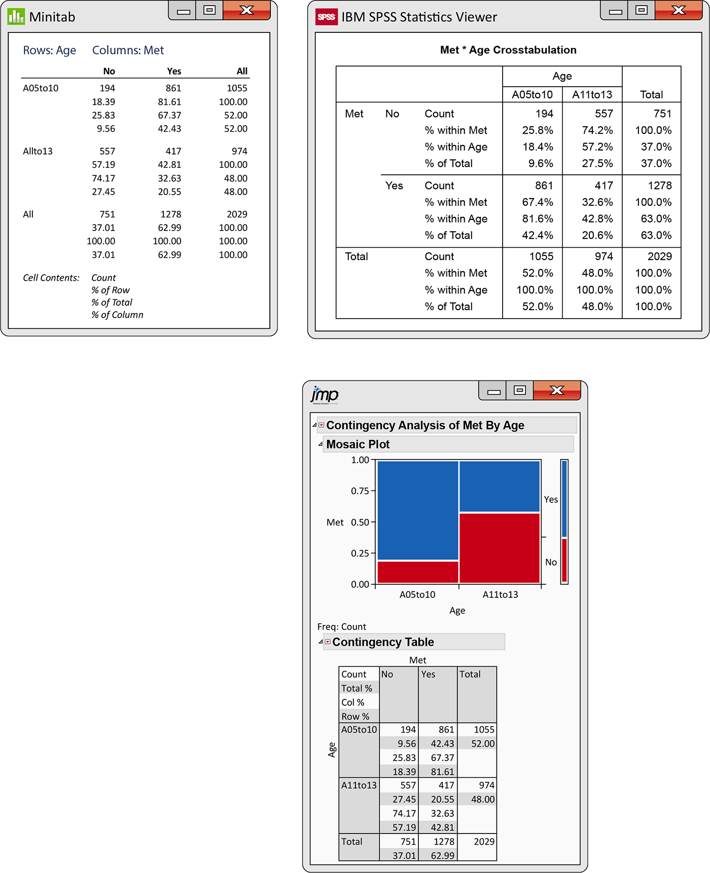
Figure 2.31 gives computer output for the data in Example 2.40 using Minitab, SPSS, and JMP. There are minor variations among software packages, but these outputs are typical of what is usually produced. Each cell in the 2×2 table has four entries. These are the count (the number of observations in the cell), the conditional distributions for rows and columns, and the joint distribution. Note that all of these are expressed as percents rather than proportions. Marginal totals and distributions are given in the rightmost column and the bottom row.

Minitab, SPSS, and JMP outputs. — Figure 2.31 Minitab, SPSS, and JMP outputs for the calcium requirement study, Example 2.47.

The Minitab output shows a contingency table with rows representing age and columns representing ideology. A key at the bottom identifies the output in each cell of the table. Each cell lists four values which represent the following, count, percentage of row, percentage of total, and percentage of column. The data is as follows. Age 5 to 10. No, 194, 18.39, 25.83, 9.56. Yes, 861, 81.61, 67.37, 42.43. All, 1055, 100.00, 52.00, 52.00. Age 11 to 13. No, 557, 57.19, 74.17, 27.45. Yes, 417, 42.81, 32.63, 20.55. All, 974, 100.00, 48.00, 48.00. Age, all. No, 751, 37.01, 100.00, 37.01. Yes, 1278, 62.99, 100.00, 62.99. Total all, 2029, 100.00, 100.00, 100.00. The SPSS shows a similar table titled, met, age crosstabulation. Rows represent met and columns represent age. A key identifies the output in each cell of the table. Each cell lists four values which represent the following, count, percentage within met, percentage within age, percentage of total. The data is as follows. Met, no. Age 5 to 10, 194, 25.8 percent, 18.4 percent, 9.6 percent. Age 11 to 13, 557, 74.2 percent, 57.2 percent, 27.5 percent. Total no, 751 100.0 percent, 37.0 percent, 37.0 percent. Met, yes. Age 5 to 10, 861, 67.4 percent, 81.6 percent, 42.4 percent. Age 11 to 13, 417, 32.6 percent, 42.8 percent, 20.6 percent. Total yes, 1278, 100.0 percent, 63.0 percent, 63.0 percent. Total age 5 to 10, 1055, 52.0 percent, 100.0 percent, 52.0 percent. Total age 11 to 13, 974, 48.0 percent, 100.0 percent, 48.0 percent. Total all, 2029, 100.0 percent, 100.0 percent, 100.0 percent. The JMP output shows two expanded dropdown list menus, contingency analysis of met by age and mosaic plot. A mosaic plot is shown. It plots met on the vertical axis, ranging from 0.00 to 1.0 in increments of 0.25, versus age on the horizontal axis, with two age groups listed. By group, the data for each is as follows. Age 5 to 10. No, from 0.00 to 0.23. Yes, from 0.24 to 1.00. Age 11 to 13. No, from 0.00 to 0.61. Yes, from 0.61 to 1.00. All values estimated. Another expanded menu, contingency table, shows a table where rows represent age and columns represent met. A key identifies the output in each cell of the table. Each cell lists four values which represent the following, count, total percentage, column percentage, row percentage. The data is as follows. Age 5 to 10. No, 194, 9.56, 25.83, 18.39. Yes, 861, 42.43, 67.37, 81.61. Total count age 5 to 10, 1055. Total percentage age 5 to 10, 52.00. Age 11 to 13. No, 557, 27.45, 74.17, 57.19. Yes, 417, 20.55, 32.63, 42.81. Total count age 11 to 13, 974. Total percentage age 11 to 13, 48.00. Total count no, 751. Total percentage no, 37.01. Total count yes, 1278. Total percentage yes, 62.99. Total count all, 2029.

Most software packages order the row and column labels numerically or alphabetically. In general, it is better to use words rather than numbers for the column labels. This sometimes involves some additional work, but it avoids the kind of confusion that can result when you forget the real values associated with each numerical value. You should verify that the entries in Figure 2.31 correspond to the calculations that we performed in Examples 2.41 through 2.46. In addition, verify the calculations for the conditional distributions of age for each value of met requirement.

The JMP output in Figure 2.31 includes a graphical display of the data called a mosaic plot. The sizes of the four boxes display joint distribution. The narrow bar to the right shows the marginal distribution of Met requirements and the widths of the vertical bars show the marginal distribution of Age. The conditional distribution of Met requirements for each Age is represented in each of these vertical bars by the heights of the blue and red sections. Notice that they always add to one.

Simpson’s paradox

As is the case with quantitative variables, the effects of lurking variables can strongly influence relationships between two categorical variables. Here is an example that demonstrates the surprises that can await the unsuspecting consumer of data.

Example 2.48 Which team had better shooters?

Statistics reported for basketball games generally include the percents of field goal baskets made for each team. Here are the raw counts for a recent game between Team A and Team B:

	Team
Outcome	A	B
Made	28	26
Missed	32	34
Shots	60	60

Team A made 28 of the 60 shots it attempted. Its success rate is 28/60, or 46.7%. Team B made 26 of the 60 shots it attempted. Its success rate is 26/60, or 43.3%. So, for this game, Team A had better shooters: 46.7% versus 43.3% for Team B.

Let’s look at the data in a little more detail. The data combined two types of field goals. Shots beyond “the arc,” a certain distance from the basket, are called 3-pointers and count for three points; other shots are called 2-pointers and count for two points. Let’s look at the data separately for 2-pointers and 3-pointers.

Example 2.49 Look at the data more carefully.

Here are the counts, broken down by the type of shot:

Outcome	2-pointers		3-pointers
Outcome	A	B	A	B
Made	25	16	3	10
Missed	25	14	7	20
Shots	50	30	10	30

Team A made 25 of the 50 2-pointers it attempted. Its success rate is 25/50, or 50.0%. Team B made 16 of the 30 2-pointers it attempted. Its success rate is 16/30, or 53.3%. So, for 2-pointers, Team B had better shooters: 53.3% versus 50.0% for Team A. On the other hand, Team A made 3 of the 10 3-pointers it attempted. Its success rate is 3/10, or 30.0%. Team B made 10 of the 30 3-pointers it attempted. Its success rate is 10/30, or 33.3%. So, for 3-pointers, Team B also had better shooters: 33.3% versus 30.0% for Team A.

The result seems strange. When looking at all field goals, Team A had better shooters in this game, but when looking at 2-pointers and 3-pointers separately, Team B shot better for both types of shots.

These results can be explained by a lurking variable (page 122): type of shot (2-pointer versus 3-pointer). Shots farther from the basket, 3-pointers, are more difficult and have a lower success rate, whereas shots closer to the basket, 2-pointers, are easier and have a higher success rate. Team A took a higher percent of their shots as the easier 2-pointers (50/60=83.3% versus Team B’s 30/60=50.0%). The higher percent of easier shots resulted in the overall success rate for Team A being higher.

The original two-way table, which did not take account of the type of shot, was misleading. This example illustrates Simpson’s paradox, an extreme form of the fact that observed associations can be misleading when there are lurking variables.

The lurking variable in our Simpson’s paradox example, type of shot, is categorical. It breaks the observations into groups by 2-pointers versus 3-pointers. In Example 2.49, these data are given in a three-way table that reports counts for each combination of three categorical variables: team, outcome, and type of shot. The three-way table is constructed from two two-way tables, one for each type of shot. The original table in Example 2.48 can be obtained by adding the corresponding cell counts for these two tables by a process known as aggregation. When we aggregated data in Example 2.48, we ignored the variable type of shot, which then became a lurking variable. caution Conclusions that seem obvious when we look only at aggregated data can become quite different when we examine the data in more detail.

Section 2.6 SUMMARY

A two-way table of counts organizes data about two categorical variables. Values of the row variable label the rows that run across the table, and values of the column variable label the columns that run down the table. Two-way tables are often used to summarize large amounts of data by grouping outcomes into categories.
The joint distribution of the row and column variables is found by dividing the count in each cell by the total number of observations.
The row totals and column totals in a two-way table give the marginal distributions of the two variables separately. It is clearer to present these distributions as percents of the table total. Marginal distributions do not give any information about the relationship between the variables.
To find the conditional distribution of the row variable for one specific value of the column variable, look only at that one column in the table. Find each entry in the column as a percent of the column total.
There is a conditional distribution of the row variable for each column in the table. Comparing these conditional distributions is one way to describe the association between the row and the column variables. It is particularly useful when the column variable is the explanatory variable. When the row variable is explanatory, find the conditional distribution of the column variable for each row and compare these distributions.
Bar graphs and mosaic plots are useful graphical displays for describing the relationship between two categorical variables.
We present data on three categorical variables in a three-way table, printed as separate two-way tables for each level of the third variable. A comparison between two variables that holds for each level of a third variable can be changed or even reversed when the data are aggregated by summing over all levels of the third variable. Simpson’s paradox refers to the reversal of a comparison by aggregation. It is an example of the potential effect of lurking variables on an observed association.

Now that you have completed this section, you will be able to:

Identify the row variable, the column variable, and the cells in a two-way table. Review Example 2.41 (page 129) and try Exercise 2.97.
Find and interpret the joint distribution in a two-way table. Review Example 2.42 (page 130) and try Exercise 2.99.
Find and interpret the marginal distributions in a two-way table. Review Example 2.43 (page 131) and try Exercise 2.99.
Use the conditional distributions to describe the relationship displayed in a two-way table. Review Example 2.46 (page 133) and try Exercise 2.99.
Determine the joint distribution, the marginal distributions, and the conditional distributions in a two-way table from software output. Review Example 2.47 (page 133) and try Exercise 2.101.
Interpret examples of Simpson’s paradox. Review Examples 2.48 and 2.49 (page 135) and try Exercises 2.105 and 2.106.

Section 2.6 EXERCISES

2.97 Does driver’s ed help? A study is planned to look at the effect of driver education programs on accidents. The driving records of all drivers under 18 in a given year will classify each driver as having taken a driver’s education course or not. The drivers will also be classified with respect to the number of accidents that they had in the year after they received their license. The categories are zero, one, and two or more accidents.
1. There are two variables in this study. Do you think one is an explanatory variable and the other is a response variable? Explain your answer.
2. Sketch a two-way table that could be used to organize the data. Which variable is the row variable? Which variable is the column variable?
3. How many cells are in the table? Describe in words what each of the cells will contain when the data are collected.
2.98 Music and video games. You are planning a study of undergraduates in which you will examine the relationship between listening to music and playing video games. The study subjects will be asked how much time they spend in each of these activities during a typical day. The choices for both activities will be a half hour or less, more than a half hour but less than an hour, and more than an hour.
1. There are two variables in this study. Do you think that one is an explanatory variable and the other is a response variable? Explain your answer.
2. Sketch a two-way table that could be used to organize the data. Which variable is the row variable? Which variable is the column variable?
3. How many cells are in the table? Describe in words what each of the cells will contain when the data are collected.

2.99 Eight is enough. A healthy body needs good food, and healthy teeth are needed to chew our food so that it can nourish our bodies. The U.S. Army has recognized this fact and requires recruits to pass a dental examination. If you wanted to be a soldier in the Spanish American War, which took place in 1898, you needed to have at least eight teeth. Here is the statement of the requirement:

Unless an applicant has at least four sound double teeth, one above and one below on each side of the mouth, and so opposed as to serve the purpose of mastication, he should be rejected.

A study reported the rejection data for enlistment candidates classified by age. Here are the data:²⁷

Rejected	Age
Rejected	Under 20	20 to 25	25 to 30	30 to 35	35 to 40	Over 40
Yes	68	647	1,114	1,783	2,887	3,801
No	58,884	77,992	55,597	43,994	47,569	39,985

Which variable is the explanatory variable? Which variable is the response variable? Give reasons for your answer.
Find the joint distribution. Write a brief summary explaining the major features of this distribution.
Find the two marginal distributions. Write a brief summary explaining the major features of these distributions.
Which conditional distribution would you choose to explain the relationship between these two variables? Explain your answer.
Find the conditional distribution that you chose in part (d), and write a summary that includes your interpretation of the relationship based on this conditional distribution.

2.100 Survival and class on the Titanic. On April 15, 1912, on her maiden voyage, the Titanic collided with an iceberg and sank. The ship was luxurious but did not have enough lifeboats for the 2224 passengers and crew. As a result of the collision, 1502 people died.²⁸ The level of luxury and the price of the ticket varied with the class, first class being the most luxurious. There were 323 passengers in first class, 277 in second class, and 709 in third class. The number of first-class passengers who survived was 200. For second- and third-class passengers who survived, the numbers were 119 and 181, respectively. Let’s look at these data with a two-way table.
1. Create a two-way table that you could use to explore the relationship between survival and class.
2. Which variable is the explanatory variable, and which is the response variable? Give reasons for your answers.
3. Find the two marginal distributions. Write a brief summary explaining the major features of these distributions.
4. Which conditional distribution would you choose to explain the relationship between these two variables? Explain your answer.
5. Find the conditional distribution that you chose in part (d) and write a summary that includes your interpretation of the relationship based on this conditional distribution.
2.101 Lying to a teacher. One of the questions in a survey of high school students asked about lying to teachers.²⁹ The data set LYING gives the numbers of students who said that they lied to a teacher about something significant at least once during the past year, classified by sex. Figure 2.32 gives software output for these data. Use this output to analyze these data and write a report summarizing your work. Be sure to include a discussion of whether or not you consider this relationship to involve an explanatory variable and a response variable.

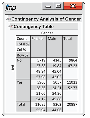
Figure 2.32 JMP output for the lying to a teacher data, Exercise 2.101.

The output shows two expanded dropdown list menus, contingency analysis of gender and contingency table. It then shows a table where rows represent lied and columns represent gender. A key identifies the output in each cell of the table. Each cell lists four values which represent the following, count, total percentage, column percentage, row percentage. The data is as follows. Lied, no. Female, 5719, 27.38, 48.94, 57.98. Male, 4145, 19.84, 45.04, 42.02. Total count no, 9864. Total percentage no, 47.23. Lied, yes. Female, 5966, 28.56, 51.06, 54.12. Male, 5057, 24.21, 54.96, 45.88. Total count yes, 11023. Total percentage yes, 52.77. Total count female, 11685. Total percentage female, 55.94. Total count male, 9202. Total percentage male, 44.06. Total count all, 20887.
2.102 Trust and honesty in the workplace. The students surveyed in the study described in the previous exercise were also asked whether they thought trust and honesty are essential in business and the workplace. Figure 2.33 gives software output for these data. Use this output to analyze these data and write a report summarizing your work. Be sure to include a discussion of whether or not you consider this relationship to involve an explanatory variable and a response variable.

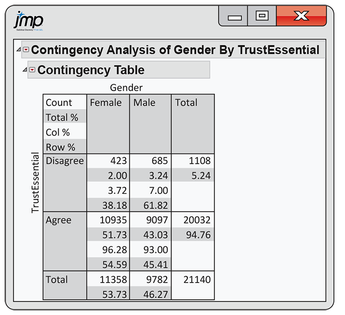
Figure 2.33 JMP output for the trust and honesty in the workplace data, Exercise 2.102.

The output shows two expanded dropdown list menus, contingency analysis of trust essential and contingency table. It then shows a table where rows represent trust essential and columns represent gender. A key identifies the output in each cell of the table. Each cell lists four values which represent the following, count, total percentage, column percentage, row percentage. The data is as follows. Trust essential, disagree. Female, 423, 2.00, 3.72, 38.18. Male, 685, 3.24, 7.00, 61.82. Total count disagree, 1108. Total percentage disagree, 5.24. Trust essential, agree. Female, 10935, 51.73, 96.28, 54.59. Male, 9097, 43.03, 93.00, 45.41. Total count agree, 20032. Total percentage agree, 94.76. Total count female, 11358. Total percentage female, 53.73. Total count male, 9782. Total percentage male, 46.27. Total count all, 21140.

2.103 Exercise and adequate sleep. A survey of 656 boys and girls, who were 13 to 18 years old, asked about adequate sleep and other health-related behaviors. The recommended amount of sleep is six to eight hours per night.³⁰ In the survey, 59% of the respondents reported that they got less than this amount of sleep on school nights. An exercise scale was developed and used to classify the students as above or below the median in this domain. Here is the 2×2 table of counts with students classified as getting or not getting adequate sleep and by the exercise variable:

Enough sleep	Exercise
Enough sleep	High	Low
Yes	151	115
No	148	242

Find the distribution of adequate sleep for the high exercisers.
Repeat part (a) for the low exercisers.
Summarize the relationship between adequate sleep and exercise using the results of parts (a) and (b).

2.104 Adequate sleep and exercise. Refer to the previous exercise.
1. Find the distribution of exercise for those who get adequate sleep.
2. Do the same for those who do not get adequate sleep.
3. Write a short summary of the relationship between adequate sleep and exercise, using the results of parts (a) and (b).
4. Compare this summary with your summary from part (c) of the previous exercise. Which do you prefer? Give a reason for your answer.

2.105 Which hospital is safer? Insurance companies and consumers are interested in the performance of hospitals. The government releases data about patient outcomes in hospitals that can be useful in making informed health care decisions. Here is a two-way table of data on the survival of patients after surgery in two hospitals. All patients undergoing surgery in a recent time period are included. “Survived” means that the patient lived at least six weeks following surgery.

	Hospital A	Hospital B
Died	63	16
Survived	2037	784
Total	2100	800

What percent of Hospital A patients died? What percent of Hospital B patients died? These are the numbers one might see reported in the media.

2.106 Patients in “poor” or “good” condition. Refer to the previous exercise. Not all surgery cases are equally serious. Patients are classified as being in either “poor” or “good” condition before surgery. Here are the data broken down by patient condition. The entries in the original two-way table are just the sums of the “poor” and “good” entries in this pair of tables.

	Good condition
	Hospital A	Hospital B
Died	6	8
Survived	594	592
Total	600	600

	Poor condition
	Hospital A	Hospital B
Died	57	8
Survived	1443	192
Total	1500	200

Find the death rate for Hospital A patients who were classified as “poor” before surgery. Do the same for Hospital B. In which hospital do “poor” patients fare better?
Repeat part (a) for patients classified as “good” before surgery.
What is your recommendation to someone facing surgery and choosing between these two hospitals?
How can Hospital A do better in both groups, yet do worse overall? Look at the data and carefully explain how this can happen.

2.107 Complete the table. Here are the row and column totals for a two-way table with two rows and two columns:

a	b	400
c	d	200
400	200	600

Find two different sets of counts a, b, c, and d for the body of the table that give these same totals. This shows that the relationship between two variables cannot be obtained from the two individual distributions of the variables.

2.108 Construct a table with no association. Construct a 2×4 table of counts where there is no apparent association between the row and column variables.