4.2 Probability Models
The idea of probability as a proportion of outcomes in very many repeated trials guides our intuition but is hard to express in mathematical form. A description of a random phenomenon in the language of mathematics is called a probability model. To see how to proceed, think first about a very simple random phenomenon: tossing a coin once. When we toss a coin, we cannot know the outcome in advance. What do we know? We are willing to say that the outcome will be either heads or tails. Because the coin appears to be balanced, we believe that each of these outcomes has probability 1/2. This description of coin tossing has two parts:
- A list of possible outcomes.
- A probability for each outcome.
This two-part description is the starting point for a probability model. We will begin by describing the outcomes of a random phenomenon and then learn how to assign probabilities to the outcomes.
Sample spaces
A probability model first tells us what outcomes are possible.
The name “sample space” is natural in random sampling, where each possible outcome is a sample, and the sample space contains all possible samples. To specify S, we must state what constitutes an individual outcome and then state which outcomes can occur. We often have some freedom in defining the sample space, so the choice of S is a matter of convenience as well as correctness. The idea of a sample space, and the freedom we may have in specifying it, are best illustrated by examples.
Example 4.6 Sample space for tossing a coin.
Toss a coin. There are only two possible outcomes, and the sample space is
or, more briefly,
Example 4.7 Sample space for random digits.
Let your pencil point fall blindly into Table B of random digits. Record the value of the digit it lands on. The possible outcomes are
Example 4.8 Sample space for tossing a coin four times.
Toss a coin four times and record the results. That’s a bit vague. To be exact, record the results of each of the four tosses in order. A typical outcome is then HTTH. Counting shows that there are 16 possible outcomes. The sample space S is the set of all 16 strings of four H’s and T’s:
Suppose that our only interest is the number of heads in four tosses. Now we can be exact in a simpler fashion. The random phenomenon is to toss a coin four times and count the number of heads. The sample space contains only five outcomes:
This example illustrates the importance of carefully specifying what constitutes an individual outcome.
Although these examples seem remote from the practice of statistics, the connection is surprisingly close. Suppose that in conducting an opinion poll, you select four people at random from a large population and ask each if he or she favors reducing federal spending on low-interest student loans. The answers are Yes or No. The possible outcomes—the sample space—are exactly as in Example 4.8 if we replace heads by Yes and tails by No. Similarly, the possible outcomes of an SRS of 1500 people are the same, in principle, as the possible outcomes of tossing a coin 1500 times. One of the great advantages of mathematics is that the essential features of quite different phenomena can be described by the same probability model.
Check-in
-
4.2 Servings of fruits and vegetables? A student is asked “How many servings of fruits and vegetables did you eat yesterday?” Set up an appropriate sample space for this setting.
The sample spaces described in Examples 4.6, 4.7, and 4.8 correspond to categorical variables where we can list all the possible values. Other sample spaces correspond to quantitative variables. Here is an example.
Example 4.9 Using software.
Most statistical software has a function that will generate a random number between 0 and 1. The sample space is
This S is a mathematical idealization. Any specific random number generator produces numbers with some limited number of decimal places so that, strictly speaking, not all numbers between 0 and 1 are possible outcomes. For example, Minitab generates random numbers like 0.736891, with six decimal places. The entire interval from 0 to 1 is easier to think about. It also has the advantage of being a suitable sample space for different software systems that produce random numbers with different numbers of digits.
Check-in
-
4.3 How much sleep? You record the number of minutes that you slept yesterday. What is the sample space?
A sample space S lists the possible outcomes of a random phenomenon. To complete a mathematical description of the random phenomenon, we must also give the probabilities with which these outcomes occur.
The true long-term proportion of any outcome—say, “exactly two heads in four tosses of a coin”—can be found only empirically, and then only approximately. How then can we describe probability mathematically? Rather than immediately attempting to give “correct” probabilities, let’s confront the easier task of laying down rules that any assignment of probabilities must satisfy. We need to assign probabilities not only to single outcomes but also to sets of outcomes.
Example 4.10 Exactly one head in four tosses.
Take the sample space S for four tosses of a coin shown in Example 4.8. Then “exactly one head” is an event. Call this event A. The event A expressed as a set of outcomes of S is
In a probability model, events have probabilities. What properties must any assignment of probabilities to events have? Here are some basic facts about any probability model. These facts follow from the idea of probability as “the long-run proportion of repetitions on which an event occurs.”
-
Any probability is a number between 0 and 1. Any proportion is a number between 0 and 1, so any probability is also a number between 0 and 1. An event with probability 0 never occurs, and an event with probability 1 occurs on every trial. An event with probability 0.5 occurs in half the trials in the long run.
-
All possible outcomes together must have probability 1. Because every trial will produce an outcome, the sum of the probabilities for all possible outcomes must be exactly 1.
-
If two events have no outcomes in common, the probability that one or the other occurs is the sum of their individual probabilities. If one event occurs in 40% of all trials, a different event occurs in 25% of all trials, and the two can never occur together, then one or the other occurs in 65% of all trials because
-
The probability that an event does not occur is 1 minus the probability that the event does occur. If an event occurs in (say) 70% of all trials, it fails to occur in the other 30%. The probability that an event occurs and the probability that it does not occur always add to 100%, or 1.
Probability rules
Formal probability uses mathematical notation to state Facts 1 through 4 more concisely. We use capital letters near the beginning of the alphabet to denote events. If A is any event, we write its probability as P(A). Here are our probability facts in formal language. As you apply these rules, remember that they are just another form of intuitively true facts about long-run proportions.
You may find it helpful to draw a picture to remind yourself of the
meaning of complements and disjoint events. A picture like
Figure 4.2
that shows the sample space S as a rectangular area and events
as areas within S is called a
Venn
diagram. The events A and B in
Figure 4.2 are
disjoint because they do not overlap. As
Figure 4.3
shows, the complement
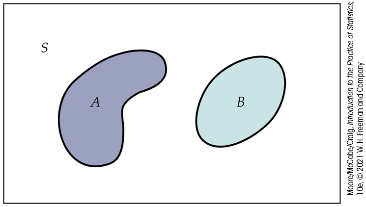
Figure 4.2 Venn diagram showing disjoint events A and B. Disjoint events have no common outcomes.
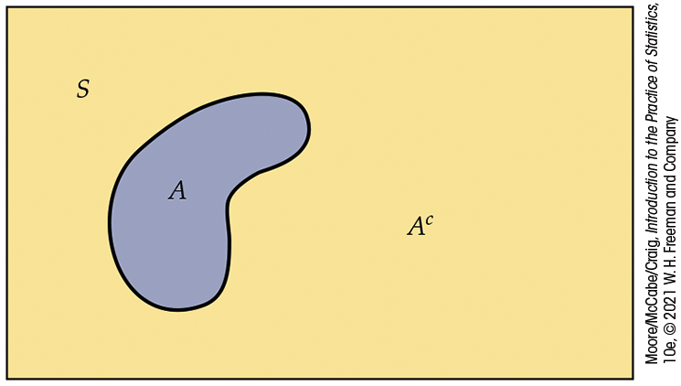
Figure 4.3 Venn diagram
showing the complement
Example 4.11 Favorite vehicle colors.
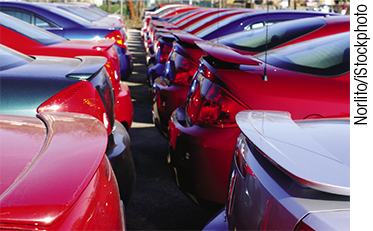
What is your favorite color for a vehicle? Our preferences can be related to our personality, our moods, or particular objects. Here is a probability model for color preferences.2
| Color | White | Black | Gray | Silver |
| Probability | 0.25 | 0.21 | 0.16 | 0.11 |
| Color | Red | Blue | Brown | Other |
| Probability | 0.10 | 0.08 | 0.04 | 0.05 |
Each probability is between 0 and 1. The probabilities add to 1 because these outcomes together make up the sample space S. Our probability model corresponds to selecting a person at random and asking what is their favorite color.
Let’s check Probability Rules 1 and 2 and use Probability Rules 3 and 4 to find some probabilities for favorite vehicle colors.
Example 4.12 Rules 1 and 2.
The probabilities for each of the colors in
Example 4.11
satisfy
Example 4.13 Black or silver?
What is the probability that a person’s favorite vehicle color is black or silver? If the favorite is black, it cannot be silver, so these two events are disjoint. Using Rule 3, we find
There is a 32% chance that a randomly selected person will choose black or silver as their favorite color.
Example 4.14 Favorite color is not blue.
To solve this problem, we could use Rule 3 and add the probabilities for white, black, silver, gray, red, brown, and other. However, it is easier to use the probability that we have for blue and Rule 4. The event that the favorite is not blue is the complement of the event that the favorite is blue. Using our notation for events, we have
We see that 92% of people have a favorite vehicle color that is not blue.
Check-in
-
4.4 Red or brown. Find the probability that the favorite color is red or brown.
-
4.5 White, black, silver, gray, or red. Find the probability that the favorite color is white, black, silver, gray, or red by using Rule 4. Explain why this calculation is easier than finding the answer by using Rule 3.
Assigning probabilities: Finite number of outcomes
The individual outcomes of a random phenomenon are always disjoint. So the addition rule for disjoint events provides a way to assign probabilities to events with more than one outcome: start with probabilities for individual outcomes and add to get probabilities for events. This idea works well when there are only a finite (fixed and limited) number of outcomes.
Example 4.15 Benford’s law.
Faked numbers in tax returns, payment records, invoices, expense account claims, and many other settings often display patterns that aren’t present in legitimate records. Some patterns, such as too many round numbers, are obvious and easily avoided by a clever crook. Others are more subtle. It is a striking fact that the first digits of numbers in legitimate records often follow a distribution known as Benford’s law. Here it is (note that a first digit can’t be 0):3
| First digit | 1 | 2 | 3 | 4 | 5 | 6 | 7 | 8 | 9 |
| Probability | 0.301 | 0.176 | 0.125 | 0.097 | 0.079 | 0.067 | 0.058 | 0.051 | 0.046 |
Benford’s law usually applies to the first digits of the sizes of similar quantities, such as invoices, expense account claims, and county populations. Investigators can detect fraud by comparing the first digits in records such as invoices paid by a business with these probabilities.
Example 4.16 Find some probabilities for Benford’s law.
Consider the events
From the table of probabilities in Example 4.15,
Note that P(B) is not the same as the probability that a first digit is strictly more than 7. The probability P(7) that a first digit is 7 is included in “7 or more” but not in “more than 7.”
Check-in
-
4.6 Benford’s law. Using the probabilities for Benford’s law, find the probability that a first digit is anything other than 9.
-
4.7 Use the addition rule. Use the addition rule with the probabilities to find the probability that a first digit is either 3 or 8 or more.
Be careful to apply the addition rule only to disjoint events.
Example 4.17 Find more probabilities for Benford’s law.
Refer to the probabilities for Benford’s law. Let D be the event that the first digit is 1, 2, or 3. Then,
Let E be the event that the first digit is 3 or 4. Then
The sum of these probabilities is
However,
which is not equal to
Check-in
-
4.8 Explain why. Refer to Example 4.17. Explain why the probability of D or E is not equal to
Assigning probabilities: Equally likely outcomes
Assigning correct probabilities to individual outcomes often requires long observation of the random phenomenon. In some circumstances, however, we are willing to assume that individual outcomes are equally likely because of some balance in the phenomenon. Ordinary coins have a physical balance that should make heads and tails equally likely, for example, and the table of random digits comes from a deliberate randomization.
Example 4.18 First digits that are equally likely.
You might think that first digits are distributed “at random” among the digits 1 to 9 in business records. The nine possible outcomes would then be equally likely. The sample space for a single digit is
Because the total probability must be 1, the probability of each of the nine outcomes must be 1/9. That is, the assignment of probabilities to outcomes is
| First digit | 1 | 2 | 3 | 4 | 5 | 6 | 7 | 8 | 9 |
| Probability |
|
|
|
|
|
|
|
|
|
The probability of the event B that a randomly chosen first digit is 7 or more is
Compare this with the Benford’s law probability in Example 4.16. A person who fakes data by using “random” digits will end up with too many first digits that are 7 or more.
In Example 4.18, all outcomes have the same probability. Because there are nine equally likely outcomes, each must have probability 1/9. Because exactly three of the nine equally likely outcomes are 7 or more, the probability of this event is 3/9. In the special situation where all outcomes are equally likely, we have a simple rule for assigning probabilities to events.
Most random phenomena do not have equally likely outcomes, so the general rule for finite sample spaces (page 215) is more important than the special rule for equally likely outcomes.
Check-in
-
4.9 Possible outcomes for rolling a die. A die has six sides with one to six spots on each side. Give the probability distribution for the six possible outcomes that can result when a fair die is rolled.
Independence and the multiplication rule
Rule 3, the addition rule for disjoint events, describes the probability that one or the other of two events A and B will occur in the special situation when A and B cannot occur together because they are disjoint. Our final rule describes the probability that both events A and B occur, again only in a special situation. More general addition and multiplication rules appear in Section 4.5, but in our study of statistics, we will need only the versions that apply to these special situations.
Suppose that you toss a fair coin twice. You are counting heads, so two events of interest are
The events A and B are not disjoint. They occur together whenever both tosses give heads. We want to compute the probability of the event {A and B} that both tosses are heads. The Venn diagram in Figure 4.4 illustrates the event {A and B} as the overlapping area that is common to both A and B.
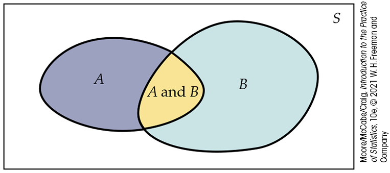
Figure 4.4 Venn diagram showing events A and B that are not disjoint. The event {A and B} consists of outcomes common to A and B.
The coin tossing of Buffon, Pearson, and Kerrich described in Example 4.3 makes us willing to assign probability 1/2 to a head when we toss a coin. So
What is P(A and B)? Our common sense says that it
is 1/4. The first toss will give a head half the time, and the second
toss will give a head half the time, so both tosses will give heads on
Our definition of independence is rather informal. We will make this informal idea precise in Section 4.5. In practice, though, we rarely need a precise definition of independence because independence is usually assumed as part of a probability model when we want to describe random phenomena that seem to be physically unrelated to each other. Here is an example of independence.
Example 4.19 Coins do not have memory.
Because a coin has no memory, we assume that coin tosses are independent. For a fair coin, this means that the outcome of the first toss does not influence the outcome of any other toss.
Check-in
-
4.10 Two heads in two tosses. What is the probability of obtaining two heads on two tosses of a fair coin?
Here is an example of a situation where there are dependent events.
Example 4.20 Dependent events in cards.
The colors of successive cards dealt from the same deck are not
independent. A standard 52-card deck contains 26 red and 26 black
cards. For the first card dealt from a shuffled deck, the
probability
of a red card is
Check-in
-
4.11 The probability of an ace. A deck of 52 cards contains 4 aces, so the probability that a card drawn from this deck is an ace is 4/52. If we know that the first card drawn is not an ace, what is the probability that the second card drawn is an ace? Using the idea of independence, explain why this probability is not 4/52.
Here is another example of a situation where events are dependent.
Example 4.21 Taking a test twice.
If you take an IQ test or other mental test twice in succession, the two test scores are not independent. The learning that occurs on the first attempt influences your second attempt. If you learn a lot, then your second test score might be a lot higher than your first test score.
When independence is part of a probability model, the multiplication rule applies. Here is an example.
Example 4.22 Mendel’s peas.
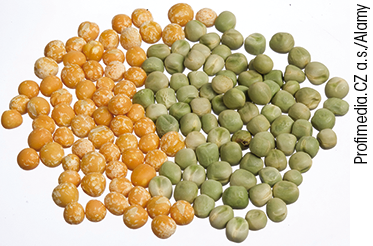
Gregor Mendel used garden peas in some of the experiments that revealed that inheritance operates randomly. The seed color of Mendel’s peas can be either green or yellow. Two parent plants are “crossed” (one pollinates the other) to produce seeds.
Each parent plant carries two genes for seed color, and each of these genes has probability 0.5 of being passed to a seed. The two genes that the seed receives, one from each parent, determine its color. The parents contribute their genes independently of each other.
Suppose that both parents carry the G and the Y genes. The seed will be green if both parents contribute a G gene; otherwise, it will be yellow. If M is the event that the male contributes a G gene and F is the event that the female contributes a G gene, then the probability of a green seed is
In the long run, 1/4 of all seeds produced by crossing these plants will be green.
![]() The multiplication rule applies only to independent events; you
cannot use it if events are not independent. Here is a distressing example of misuse of the multiplication rule.
The multiplication rule applies only to independent events; you
cannot use it if events are not independent. Here is a distressing example of misuse of the multiplication rule.
Example 4.23 Sudden infant death syndrome.
Sudden infant death syndrome (SIDS) causes babies to die suddenly (often in their cribs) with no explanation. Deaths from SIDS have been greatly reduced by placing babies on their backs, but as yet no cause for SIDS is known.
When more than one SIDS death occurs in a family, the parents are sometimes accused. One “expert witness” popular with prosecutors in England told juries that there is only a 1 in 73 million chance that two children in the same family could have died from SIDS. Here’s his calculation: the rate of SIDS in a nonsmoking middle-class family is 1 in 8500. So the probability of two deaths is
Several women were convicted of murder on this basis, without any direct evidence that they had harmed their children.
As the Royal Statistical Society said, this reasoning is nonsense. It assumes that SIDS deaths in the same family are independent events. The cause of SIDS is unknown: “There may well be unknown genetic or environmental factors that predispose families to SIDS, so that a second case within the family becomes much more likely.”4 The British government decided to review the cases of 258 parents convicted of murdering their babies.
The multiplication rule
![]() You must also be certain not to confuse disjointness and
independence. Disjoint events cannot be independent.
If A and B are disjoint, then the fact that
A occurs tells us that B cannot occur; look again at
Figure 4.2 (page 213). Unlike disjointness or complements, independence cannot be
pictured by a Venn diagram because it involves the probabilities of
the events rather than just the outcomes that make up the events.
However, it could be displayed in a mosaic plot.
You must also be certain not to confuse disjointness and
independence. Disjoint events cannot be independent.
If A and B are disjoint, then the fact that
A occurs tells us that B cannot occur; look again at
Figure 4.2 (page 213). Unlike disjointness or complements, independence cannot be
pictured by a Venn diagram because it involves the probabilities of
the events rather than just the outcomes that make up the events.
However, it could be displayed in a mosaic plot.
Applying the probability rules
If two events A and B are independent, then their
complements
The multiplication rule also extends to collections of more than two events, provided that all are independent. Independence of events A, B, and C means that no information about any one or any two can change the probability of the remaining events. The formal definition is a bit messy. Fortunately, independence is usually assumed in setting up a probability model. We can then use the multiplication rule freely.
By combining the rules we have learned, we can compute probabilities for rather complex events. Here is an example.
Example 4.24 HIV testing.
Many people who come to clinics to be tested for HIV, the virus that causes AIDS, don’t come back to learn the test results. Clinics now use “rapid HIV tests” that give a result in a few minutes. The false-positive rate for a diagnostic test is the probability that a person with no disease will have a positive test result. For the rapid HIV tests, the Food and Drug Administration (FDA) has established 2% as the maximum false-positive rate allowed for a rapid HIV test.5 If a clinic uses a test that matches the FDA standard and tests 50 people who are free of HIV antibodies, what is the probability that at least one false-positive will occur?
It is reasonable to assume as part of the probability model that
the test results for different individuals are independent. The
probability that the test is positive for a single person is 0.02,
so the probability of a negative result is
There is approximately a 64% chance that at least 1 of the 50 people will test positive for HIV even though those people do not have the virus.
Concern about excessive numbers of false-positives led the New York City Department of Health and Mental Hygiene to suspend the use of one particular rapid HIV test.6
Section 4.2 SUMMARY
-
A probability model for a random phenomenon consists of a sample space S and an assignment of probabilities P.
-
The sample space S is the set of all possible outcomes of the random phenomenon. Sets of outcomes are called events. P assigns a number P(A) to an event A as its probability.
-
The complement
-
Any assignment of probability must obey the rules that state the basic properties of probability:
-
Rule 1.
-
Rule 2.
-
Rule 3. Addition rule: If events A and B are disjoint, then
-
Rule 4. Complement rule: For any event A,
-
Rule 5. Multiplication rule: If events A and B are independent, then
-
Section 4.2 EXERCISES
-
4.8 What is the sample space? You toss a fair coin five times.
-
What is the sample space if you record the result of each toss (H or T)?
-
What is the sample space if you record the number of heads?
-
-
4.9 Define the sample space. For each of the following questions, define a sample space for the associated random phenomenon. Explain your answers. Be sure to specify units if that is appropriate.
-
How many people do you talk with in a typical day?
-
How much did you spend on textbooks this semester?
-
If you Google the word “statistics,” how long will it take for you to receive a response?
Will it snow tomorrow?
-
-
4.10 What’s wrong? In each of the following scenarios, there is something wrong. Describe what is wrong and give a reason for your answer.
-
If the probability of A is 0.6 and the probability of B is 0.7, the probability of both A and B happening is 1.3.
-
If the probability of A is 0.55, then the probability of the complement of A is
-
If two events are disjoint, we can multiply their probabilities to determine the probability that they will both occur.
-
-
4.11 Probability rules. For each of the following situations, state the probability rule or rules that you would use and apply it or them. Write a sentence explaining how the situation illustrates the use of the probability rules.
-
A coin is tossed three times. The probability of zero heads is 1/8, and the probability of zero tails is 1/8. What is the probability that all three tosses result in the same outcome?
-
Refer to part (a). What is the probability that there is at least one head and at least one tail?
-
The probability of event A is 0.5, and the probability of event B is 0.9. Events A and B are disjoint. Can this happen?
-
Event A is very rare. Its probability is
-
The probability of event A is 0.23. What is the probability that event A does not occur?
-
You toss a coin two times. It is not a fair coin, and you do not know the probability of a head. What is the probability that either zero, one, or two heads appear?
-
-
4.12 The multiplication rule for independent events. The probability that a randomly selected person prefers the vehicle color white is 0.25. Can you apply the multiplication rule for independent events in the situations described in parts (a) and (b)? If your answer is Yes, apply the rule.
-
Two people are chosen at random from the population. What is the probability that both prefer white?
-
Two people who are sisters are chosen. What is the probability that both prefer white?
-
Write a short summary about the multiplication rule for independent events using your answers to parts (a) and (b) to illustrate the basic idea.
-
-
4.13 Equally likely events. For each of the following situations, explain why you think that the events are equally likely or not. Explain your answers.
-
You roll a fair die and get an even number or an odd number.
-
You are observing cars at an intersection. You classify the movement of each car as a right turn, a left turn, or straight through the intersection.
-
For college basketball games, you record the times that the home team wins and the number of times that the home team loses.
-
The outcome of the next tennis match for Ashleigh Barty is either a win or a loss.
-
-
4.14 What’s wrong? In each of the following scenarios, there is something wrong. Describe what is wrong and give a reason for your answer.
-
If we select a digit at random, then the probability of selecting a 4 is 0.4.
-
If the probability of A is 0.2, the probability of B is 0.3, and the probability of A and B is 0.5, then A and B are independent.
-
If the sample space consists of four outcomes, then each outcome has probability 0.25.
-
-
4.15 Evaluating web page designs. You are a web page designer, and you set up a page with four different links. A user of the page can click on one of the links, or he or she can leave that page. Describe the sample space for the outcome of someone visiting your web page.
-
4.16 Record the length of time spent on the page. Refer to the previous exercise. You also decide to measure the length of time a visitor spends on your page. Give the sample space for this measure.
-
4.17 Distribution of blood types. All human blood can be “ABO-typed” as one of O, A, B, or AB, but the distribution of the types varies a bit among groups of people. Here is the distribution of blood types for a randomly chosen person in the United States:7
Blood type A B AB O U.S. probability 0.42 0.11 0.03 ? -
What is the probability of type O blood in the United States?
-
Sasha has type A blood. She can safely receive blood transfusions from people with blood types O and A. What is the probability that a randomly chosen person from the United States can donate blood to Sasha? (This exercise and the one that follows ignore the Rh factor, another classification of blood types that is related to whether one person can donate blood to another.)
-
-
4.18 Blood types in Ireland. The distribution of blood types in Ireland differs from the U.S. distribution given in the previous exercise:
Blood type A B AB O Ireland probability 0.35 0.10 0.03 0.52 Choose a person from the United States and a person from Ireland at random, independently of each other. What is the probability that both have type O blood? What is the probability that both have the same blood type?
-
4.19 Are the probabilities legitimate? In each of the following situations, state whether or not the given assignment of probabilities to individual outcomes is legitimate—that is, whether it satisfies the rules of probability. If not, give specific reasons for your answer.
-
Deal a card from a shuffled deck:
-
Roll a die and record the count of spots on the up-face:
-
Choose a college student at random and record gender and enrollment status:
-
-
4.20 French and English in Canada. Canada has two official languages, English and French. Choose a Canadian at random and ask, “What is your mother tongue?” Here is the distribution of responses:8
Language English French Other Probability 0.56 0.21 ? -
What probability should replace “?” in the distribution?
-
What is the probability that a Canadian’s mother tongue is not English? Explain how you computed your answer.
-
-
4.21 Education levels of young adults. Choose a young adult (age 25 to 34 years) at random. The probability is 0.12 that the person chosen did not complete high school, 0.31 that the person has a high school diploma but no further education, and 0.29 that the person has at least a bachelor’s degree.
-
What must be the probability that a randomly chosen young adult has some education beyond high school but does not have a bachelor’s degree?
-
What is the probability that a randomly chosen young adult has at least a high school education?
-
-
4.22 Loaded dice. There are many ways to produce crooked dice. To load a die so that 6 comes up too often and 1 (which is opposite 6) comes up too seldom, add a bit of lead to the spot on the 1 face. Because the spot is solid plastic, this works even with transparent dice. If a die is loaded so that 6 comes up with probability 0.24 and the probabilities of the 2, 3, 4, and 5 faces are not affected, what is the assignment of probabilities to the six faces?
-
4.23 Rh blood types. Human blood is typed as O, A, B, or AB and also as Rh-positive or Rh-negative. ABO type and Rh-factor type are independent because they are governed by different genes. In the American population, 84% of people are Rh-positive. Use the information about ABO type in Exercise 4.17 to give the probability distribution of blood type (ABO and Rh) for a randomly chosen American.
-
4.24 Roulette. A roulette wheel has 38 slots, numbered 0, 00, and 1 to 36. The slots 0 and 00 are colored green, 18 of the others are red, and 18 are black. The dealer spins the wheel and, at the same time, rolls a small ball along the wheel in the opposite direction. The wheel is carefully balanced so that the ball is equally likely to land in any slot when the wheel slows. Gamblers can bet on various combinations of numbers and colors.
-
What is the probability that the ball will land in any one slot?
-
If you bet on “red,” you win if the ball lands in a red slot. What is the probability of winning?
-
The slot numbers are laid out on a board on which gamblers place their bets. One column of numbers on the board contains all multiples of 3—that is, 3, 6, 9, . . . , 36. You place a “column bet” that wins if any of these numbers comes up. What is your probability of winning?
-
-
4.25 Winning the lottery. A state lottery’s Pick 3 game asks players to choose a three-digit number, 000 to 999. The state chooses the winning three-digit number at random so that each number has probability 1/1000. You win if the winning number contains the digits in your number, in any order.
-
Your number is 059. What is your probability of winning?
-
Your number is 223. What is your probability of winning?
-
-
4.26 PINs. The personal identification numbers (PINs) for automatic teller machines usually consist of four digits. You notice that most of your PINs have at least one 0, and you wonder if the issuers use lots of 0s to make the numbers easy to remember. Suppose that PINs are assigned at random, so that all four-digit numbers are equally likely.
How many possible PINs are there?
-
What is the probability that a PIN assigned at random has at least one 0?
-
4.27 Universal blood donors. People with type O-negative blood are universal donors. That is, any patient can receive a transfusion of O-negative blood. Only 7% of the American population have O-negative blood. If six people appear at random to give blood, what is the probability that at least one of them is a universal donor?
-
 4.28 Axioms of probability. Show that any
assignment of probabilities to events that obeys Rules 2 and 3
on
page 213
automatically obeys the complement rule (Rule 4). This implies
that a mathematical treatment of probability can start from just
Rules 1, 2, and 3. These rules are sometimes called
axioms of probability.
4.28 Axioms of probability. Show that any
assignment of probabilities to events that obeys Rules 2 and 3
on
page 213
automatically obeys the complement rule (Rule 4). This implies
that a mathematical treatment of probability can start from just
Rules 1, 2, and 3. These rules are sometimes called
axioms of probability.
-
4.29 Independence of complements.
Show that if events A and B obey the
multiplication rule,
Mendelian inheritance. Some traits of plants and animals depend on inheritance of a single gene. This is called Mendelian inheritance, after Gregor Mendel (1822–1884). Exercises 4.30 through 4.33 are based on the following information about Mendelian inheritance of blood type.
Each of us has an ABO blood type, which describes whether two characteristics, called A and B, are present. Every one of us has two blood type alleles (gene forms): one inherited from our mother and one from our father. Each of these alleles can be A, B, or O. Which two we inherit determines our blood type. Here is a table that shows what our blood type is for each combination of two alleles:
Alleles inherited Blood type A and A A A and B AB A and O A B and B B B and O B O and O O We inherit each of a parent’s two alleles with probability 0.5. We inherit independently from our mother and father.
-
4.30 Blood types of children. Emily and Michael both have alleles O and O.
What blood types can their children have?
-
What is the probability that their next child has each of these blood types?
-
4.31 Parents with alleles A and O. Andreona and Caleb both have alleles A and O.
What blood types can their children have?
-
What is the probability that their next child has each of these blood types?
-
4.32 Two children. Samantha has alleles B and O. Dylan has alleles A and B. They have two children. What is the probability that both children have blood type A? What is the probability that both children have the same blood type?
-
4.33 Three children. Anna has alleles B and O. Nathan has alleles A and O.
-
What is the probability that a child of these parents has blood type O?
-
If Anna and Nathan have three children, what is the probability that all three have blood type O? What is the probability that the first child has blood type O and the next two do not?
-