4.3 Random Variables
Sample spaces need not consist of numbers. When we toss a coin four
times, we can record the outcome as a string of heads and tails, such as
HTTH. In statistics, however, we are most often interested in numerical
outcomes such as the count of heads in the four tosses. It is convenient
to use a shorthand notation: Let X be the number of heads in four
tosses. If our outcome is HTTH, then
In this coin-tossing example, the random variable is the number of
heads in the four tosses. We usually denote random variables by capital
letters near the end of the alphabet, such as X or Y. Of
course, the random variables of greatest interest to us are outcomes
such as the mean
To consider the random variable X as a probability model, we need to describe its sample space S and a probability for each outcome. The sample space S is the list of possible values of the random variable. We usually do not mention S separately. There are two main ways of assigning probabilities to the values of a random variable, and the one we use depends on what type of random variable it is.
Discrete random variables
We have learned several rules of probability but only one method of assigning probabilities: state the probabilities of the individual outcomes and assign probabilities to events by summing over the outcomes. The outcome probabilities must be between 0 and 1 and have sum 1. When the outcomes are numerical, they are values of a random variable. We will now attach a name to random variables having probability assigned in this way.
In most discrete random variable situations that we will study, the
number of possible values is a finite number k. For example,
the number of heads in four tosses of a coin has
There are, however, other settings in which the number of possible values can be countably infinite. We’d assign most of the probability to the small values, but each toss would have a nonzero probability, and the collection of these would sum to one. Think about tossing a fair coin until you get a head. The number of possible tosses is any positive integer.
Example 4.25 Grade distributions.
A liberal arts college posts the grade distributions for its
courses. In a recent semester, students in one section of English
130 received 34% A’s, 42% B’s, 18% C’s, 2% D’s, and 4% F’s. Choose
an English 130 student
at random. To “choose at random” means to give every student the
same chance to be chosen. The student’s grade on a five-point scale
(with
The value of X changes when we repeatedly choose a student at random, but it is always one of 0, 1, 2, 3, or 4. Here is the distribution of X:
| Value of X | 0 | 1 | 2 | 3 | 4 |
| Probability | 0.04 | 0.02 | 0.18 | 0.42 | 0.34 |
The probability that the sampled student got a B or better is the sum of the probabilities of an A and a B. In the language of random variables,
Check-in
-
4.12 Will the course satisfy the requirement? Refer to Example 4.25. Suppose that a grade of D or F in English 130 will not satisfy a requirement for a major in linguistics. What is the probability that a randomly selected student will not satisfy this requirement?
We can use histograms to show not only distributions of data but also probability distributions. Here is an example.
Example 4.26 Random digit distributions.
Let’s compare the distribution of random digits with the distribution of the probability model for Benford’s law (Example 4.15) using probability histograms. Figure 4.5 displays the result.
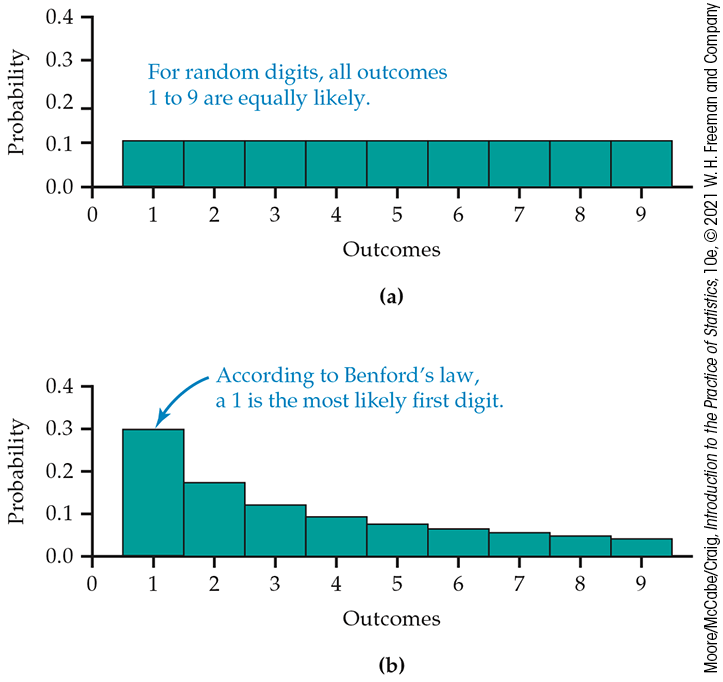
Figure 4.5 Probability histograms for (a) equally likely random digits 1 to 9 and (b) Benford’s law. The height of each bar shows the probability assigned to a single outcome.
The height of each bar shows the probability of the outcome at its base. Because the heights are probabilities, they add to 1. As usual, all the bars in a histogram have the same width. So the areas also display the assignment of probability to outcomes. Think of these histograms as idealized pictures of the results of very many trials. The histograms make it easy to quickly compare the two probability distributions.
Example 4.27 Number of heads in four tosses of a coin.
What is the probability distribution of the discrete random variable X that counts the number of heads in four tosses of a coin? We can derive this distribution if we make two reasonable assumptions:
- The coin is balanced, so it is fair, and each toss is equally likely to give H or T.
- The coin has no memory, so tosses are independent.
The outcome of four tosses is a sequence of heads and tails. There are 16 possible outcomes in all. Figure 4.6 compiles these outcomes with their values of X to represent the probability distribution of X. For the probabilities we can use the multiplication rule for independent events. For example,
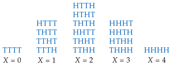
Figure 4.6 Possible outcomes in four tosses of a coin, Example 4.27. The outcomes are arranged by the values of the random variable X, the number of heads.
Similarly, each of the 16 possible outcomes has probability 1/16. That is, these outcomes are equally likely.
The number of heads X has possible values 0, 1, 2, 3, and 4.
These values are not equally likely. As
Figure 4.6
shows, there is only one way that
The event
We can find the probability of each value of X in Figure 4.6 in the same way. Here is the result:
| Value of X | 0 | 1 | 2 | 3 | 4 |
| Probability | 0.0625 | 0.25 | 0.375 | 0.25 | 0.0625 |
Figure 4.7 is a probability histogram for the distribution in Example 4.27. The probability distribution is exactly symmetric. The probabilities (bar heights) are idealizations of the proportions after very many tosses of four coins. The actual distribution of proportions observed would be nearly symmetric but is unlikely to be exactly symmetric.
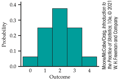
Figure 4.7 Probability histogram for the number of heads in four tosses of a coin.
Any event involving the number of heads observed in four tosses can be expressed in terms of X, and its probability can be found from the distribution of X. Here is an example.
Example 4.28 Probability of at least three heads.
The probability of tossing at least three heads is
The probability of at least one head is most simply found by use of the complement rule:
Recall that tossing a coin n times is similar to choosing an SRS of size n from a large population and asking a Yes or No question (page 211). We will extend the results of Examples 4.27 and 4.28 when we discuss sampling distributions in the next chapter.
Check-in
-
4.13 Three tosses of a fair coin. Find the probability distribution for the number of heads that appear in three tosses of a fair coin. Note: Start by finding the sample space S.
Continuous random variables
![]()
When we use the table of random digits to select a digit between 0 and 9, the result is a discrete random variable. The probability model assigns probability 1/10 to each of the 10 possible outcomes. Suppose that we want to choose a number at random between 0 and 1, allowing any number between 0 and 1 as the outcome. Software random number generators will do this. In fact, we used the Excel function RAND() for our randomization examples in Chapter 3.
You can visualize such a random number by thinking of a spinner (Figure 4.8) that turns freely on its axis and slowly comes to a stop. The pointer can come to rest anywhere on a circle that is marked from 0 to 1. The sample space is now an entire interval of numbers:
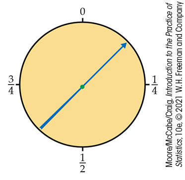
Figure 4.8 A spinner that generates a random number between 0 and 1.
How can we assign probabilities to events such as
Example 4.29 Uniform random numbers.
The random number generator will spread its output uniformly across the entire interval from 0 to 1 as we allow it to generate a long sequence of numbers. The results of many trials are represented by the density curve of a uniform distribution.
This density curve is shown in Figure 4.9. It has height 1 over the interval from 0 to 1 and height 0 everywhere else. The area under the density curve is 1: the area of a square with base 1 and height 1. The probability of any event is the area under the density curve and above the event in question.
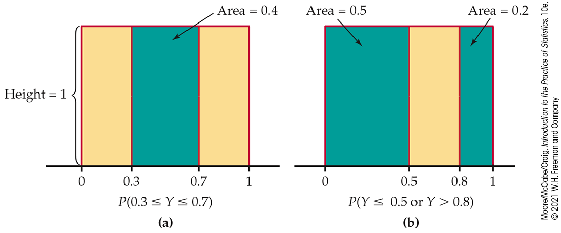
Figure 4.9 Assigning probabilities for generating a random number between 0 and 1, Example 4.29. The probability of any interval of numbers is the area above the interval and under the density curve.
Example 4.30 A uniform probability.
What is the probability that the random number generator produces a number X between 0.3 and 0.7? The answer is illustrated in Figure 4.9(a). Because the area under the density curve and above the interval from 0.3 to 0.7 is 0.4,
The height of the density curve is 1, and the area of a rectangle is the product of height and length, so the probability of any interval of outcomes is just the length of the interval.
Similarly,
Notice that the last event consists of two nonoverlapping intervals, so the total area above the event is found by adding two areas, as illustrated by Figure 4.9(b). This assignment of probabilities obeys all of our rules for probability.
Check-in
-
4.14 Find a uniform probability. For the uniform distribution described in Examples 4.29 and 4.30, find the probability that X is between 0.4 and 0.8.
Probabilities of events as areas under a density curve is our second important way of assigning probabilities. Figure 4.10 illustrates this idea in general form. We call X in Figures 4.9 and 4.10 a continuous random variable because its values are not isolated numbers but an entire interval of numbers.
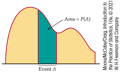
Figure 4.10 The probability distribution of a continuous random variable assigns probabilities as areas under a density curve. The total area under any density curve is 1.
The probability model for a continuous random variable assigns
probabilities to intervals of outcomes rather than to individual
outcomes. In fact,
all continuous probability distributions assign probability 0 to
every individual outcome.
Only intervals of values have positive probability. To see that this
is true, consider a specific outcome such as
Although this fact may seem odd, it makes intuitive, as well as mathematical, sense. A random number generator produces a number between 0.79 and 0.81 with probability 0.02. An outcome between 0.799 and 0.801 has probability 0.002. A result between 0.799999 and 0.800001 has probability 0.000002. You see that as this interval closes in on 0.8, the probability gets closer to 0.
To be consistent, the probability of an outcome exactly equal
to 0.8 must be 0. Because there is no probability exactly at
![]() We can ignore the distinction between
We can ignore the distinction between
Normal distributions as probability distributions
The density curves that are most familiar to us are the Normal curves.
Because any density curve describes an assignment of probabilities,
Normal distributions are continuous probability distributions.
Recall that
is a standard Normal random variable having the distribution
Example 4.31 A Normal distribution calculation.
Suppose X is a random variable with the
In terms of Z, a standard Normal random variable, we have
Using software or
Table A, we find
Check-in
-
4.15 Find a Normal probability. Refer to Example 4.31. Without doing any additional calculations, what is the probability that X is less than 15? Explain how you determined your answer.
Here’s a Normal distribution calculation that relates to the discussion of sampling distributions in the next chapter. It is also a more realistic example in that it addresses the uncertainty in a sample survey.
Example 4.32 Texting while driving.
Texting while driving can be dangerous, but many people have a hard time putting down the phone. Suppose that 26% of teen drivers text while driving. If we take a sample of 500 teen drivers, what percent would we expect to say that they text while driving?10
The proportion
We will see in the next chapter that in this setting, with teen
drivers answering honestly,
What is the probability that the survey result differs from the
truth about the population by no more than 3 percentage points? We
can use what we learned about Normal distribution calculations to
answer this question. Because
Figure 4.11 shows this probability as an area under a Normal density curve. You can find it by using software or by standardizing and using Table A. From Table A,
About 87% of the time, the sample
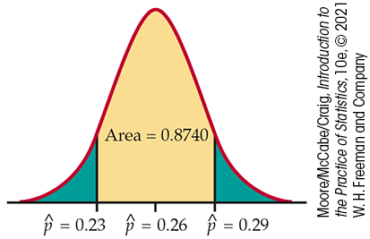
Figure 4.11 Probability as area under a Normal density curve, Example 4.32.
We began this chapter with a general discussion of the idea of probability and the properties of probability models. Two very useful specific types of probability models are distributions of discrete and continuous random variables. In our study of statistics, we will employ only these two types of probability models.
Section 4.3 SUMMARY
-
A random variable is a variable taking numerical values determined by the outcome of a random phenomenon. The probability distribution of a random variable X tells us what the possible values of X are and how probabilities are assigned to those values.
-
A random variable X and its distribution can be discrete or continuous.
-
A discrete random variable has possible values that can be given in an ordered list. The probability distribution assigns each of these values a probability between 0 and 1 such that the sum of all the probabilities is exactly 1. The probability of any event is the sum of the probabilities of all the values that make up the event.
-
A continuous random variable takes all values in some interval of numbers. A density curve describes the probability distribution of a continuous random variable. The probability of any event is the area under the curve and above the values that make up the event.
-
Uniform distributions are continuous probability distributions that are very similar to equally likely discrete distributions.
-
Normal distributions are one type of continuous probability distribution.
-
You can picture a probability distribution by drawing a probability histogram in the discrete case or by graphing the density curve in the continuous case.
Section 4.3 EXERCISES
-
4.34 A random variable? You toss two coins and record the outcome as HH, HT, TH, or TT. Is the outcome a random variable? Explain your answer.
-
4.35 How many courses? At a small liberal arts college, students can register for one to six courses. Let X be the number of courses taken in the fall by a randomly selected student from this college. In a typical fall semester, 6% take one course, 6% take two courses, 12% take three courses, 20% take four courses, 41% take five courses, and 15% take six courses. Let X be the number of courses taken in the fall by a randomly selected student from this college. Describe the probability distribution of this random variable.
-
4.36 A new random variable. Refer to the previous exercise. Suppose that a student earns three credits for each course taken. Let Y equal the number of credits a student would earn if they complete the course.
-
What is the distribution of Y?
-
Use a probability histogram to describe the distribution of Y.
-
-
4.37 Make a graphical display. Refer to Exercise 4.35. Use a probability histogram to provide a graphical description of the distribution of X.
-
4.38 Find some probabilities. Refer to Exercise 4.36.
-
Find the probability that a randomly selected student earns more than 18 credits.
-
Find the probability that a randomly selected student earns 6 or fewer credits.
-
Find the probability that a randomly selected student earns 15 credits or more.
-
-
4.39 Find more probabilities. Refer to Exercise 4.35.
-
Find the probability that a randomly selected student takes two or fewer courses.
-
Find the probability that a randomly selected student takes three or four courses.
-
Find the probability that a randomly selected student takes seven courses.
-
-
4.40 What’s wrong? In each of the following scenarios, there is something wrong. Describe what is wrong and give a reason for your answer.
-
The possible values for a discrete random variable can’t be negative.
-
A continuous random variable can take any value between 0 and 1.
-
Normal distributions are discrete random variables.
-
-
4.41 Use the uniform distribution. Suppose that a random variable X follows the uniform distribution described in Example 4.29 (page 229). For each of the following events, find the probability and illustrate your calculations with a sketch of the density curve similar to the ones in Figure 4.9 (page 229).
-
The probability that X is less than 0.2.
-
The probability that X is greater than or equal to 0.7.
-
The probability that X is less than 0.8 and greater than 0.4.
-
The probability that X is 0.7.
-
-
4.42 Use of Twitter. Suppose that the population proportion of Internet users who say that they use Twitter or another service to post updates about themselves or to see updates about others is 19%.11 Think about selecting random samples from a population in which 19% are Twitter users.
-
Describe the sample space for selecting a single person.
-
If you select three people, describe the sample space.
-
Using the results of part (b), define the sample space for the random variable that expresses the number of Twitter users in the sample of size 3.
-
What information is contained in the sample space for part (b) that is not contained in the sample space for part (c)? Do you think this information is important? Explain your answer.
-
-
4.43 Use the Normal distribution. Suppose X is a Normal random variable with mean 20 and standard deviation 4. Find the following probabilities.
-
The probability that X greater than or equal to 22.
-
The probability that X less than 22.
-
The probability that X greater than 22 and less than 24.
-
The probability that X greater than 40.
-
-
4.44 Probabilities for Twitter. Refer to the Exercise 4.42. Find the probabilities for the number of Twitter users in a sample of size 2.
-
4.45 Households and families in government data. In government data, a household consists of all occupants of a dwelling unit, while a family consists of two or more persons who live together and are related by blood or marriage. So all families form households, but some households are not families. Here are the distributions of household size and of family size in the United States:
Number of persons 1 2 3 4 5 6 7 Household probability 0.27 0.33 0.16 0.14 0.06 0.03 0.01 Family probability 0 0.44 0.22 0.20 0.09 0.03 0.02 Make probability histograms for these two discrete distributions, using the same scales. What are the most important differences between the sizes of households and families?
-
4.46 Discrete or continuous. In each of the following situations, decide whether the random variable is discrete or continuous and give a reason for your answer.
-
Your web page has five different links, and a user can click on one of the links or can leave the page. You record the length of time that a user spends on the web page before clicking one of the links or leaving the page.
-
You record the number of hits per day on your web page.
-
You record the yearly income of a visitor to your web page.
-
-
4.47 Texas hold ’em. The game Texas hold ’em starts with each player receiving two cards. Here is the probability distribution for the number of aces in two-card hands:
Number of aces 0 1 2 Probability 0.8507 0.1448 0.0045 -
Verify that this assignment of probabilities satisfies the requirement that the sum of the probabilities for a discrete distribution must be 1.
-
Make a probability histogram for this distribution.
-
What is the probability that a hand contains at least one ace? Show two different ways to calculate this probability.
-
-
4.48 Tossing two dice. Some games of chance rely on tossing two dice. Each die has six faces, marked with one, two, . . . , six spots called pips. The dice used in casinos are carefully balanced so that each face is equally likely to come up. When two dice are tossed, each of the 36 possible pairs of faces is equally likely to come up. The outcome of interest to a gambler is the sum of the pips on the two up-faces. Call this random variable X.
Write down all 36 possible pairs of up-faces.
-
If all pairs have the same probability, what must be the probability of each pair?
-
Write the value of X next to each pair of up-faces and use this information with the result of part (b) to give the probability distribution of X. Draw a probability histogram to display the distribution.
-
One bet available in the game called craps wins if a 7 or an 11 comes up on the next roll of two dice. What is the probability of rolling a 7 or an 11 on the next roll?
-
Several bets in craps lose if a 7 is rolled. If any outcome other than 7 occurs, these bets either win or continue to the next roll. What is the probability that anything other than a 7 is rolled?
-
 4.49 Nonstandard dice.
Nonstandard dice can produce interesting distributions of
outcomes. You have two balanced, six-sided dice. One is a
standard die, with faces having one, two, three, four, five, and
six spots. The other die has three faces with two spots and
three faces with five spots. Find the probability distribution
for the total number of spots Y on the up-faces when you
roll these two dice.
4.49 Nonstandard dice.
Nonstandard dice can produce interesting distributions of
outcomes. You have two balanced, six-sided dice. One is a
standard die, with faces having one, two, three, four, five, and
six spots. The other die has three faces with two spots and
three faces with five spots. Find the probability distribution
for the total number of spots Y on the up-faces when you
roll these two dice.
-
4.50 Spell-checking software. Spell-checking software catches “nonword errors,” which are strings of letters that are not words, as when “the” is typed as “eth.” When undergraduates are asked to write a 250-word essay (without spell-checking), the number X of nonword errors has the following distribution:
Value of X 0 1 2 3 4 Probability 0.2 0.4 0.2 0.1 0.1 -
Sketch the probability distribution for this random variable.
-
Write the event “at least one nonword error” in terms of X. What is the probability of this event?
-
Describe the event
-
-
4.51 Find the probabilities. Let the random variable X be a random number with the uniform density curve in Figure 4.9 (page 229). Find the following probabilities:
-
-
-
-
-
X is not in the interval 0.5 to 0.8.
-
-
4.52 Uniform numbers between 0 and 4. Many random number generators allow users to specify the range of the random numbers to be produced. Suppose that you specify that the range is to be all numbers between 0 and 4. Call the random number generated Y. Then the density curve of the random variable Y has constant height between 0 and 4 and height 0 elsewhere.
-
What is the height of the density curve between 0 and 4? Draw a graph of the density curve.
-
Use your graph from part (a) and the fact that probability is area under the curve to find
-
Find
-
Find
-
-
4.53 The sum of two uniform random numbers.
Generate two random numbers between 0 and 1 and take
Y to be their sum. Then Y is a continuous random
variable that can take any value between 0 and 2. The density
curve of Y is the triangle shown in
Figure 4.12.
-
Verify by geometry that the area under this curve is 1.
-
What is the probability that Y is less than 1? Sketch the density curve, shade the area that represents the probability, and find that area. Do this for part (c) also.
-
What is the probability that Y is greater than 1.5?
-
What is the probability that Y is greater than 0.5?
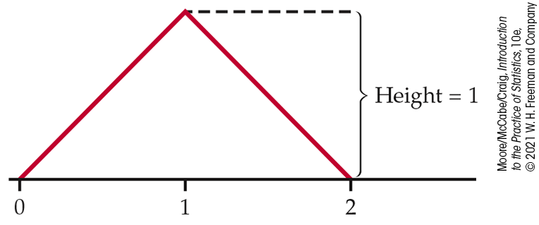
Figure 4.12 The density curve for the sum Y of two random numbers, Exercise 4.53.
-
-
4.54 How many close friends? How many close friends do you have? Suppose that the number of close friends adults claim to have varies from person to person with mean
-
4.55 Normal approximation for a sample proportion. A sample survey contacted an SRS of 700 registered voters in Oregon shortly after an election and asked respondents whether they had voted. Voter records show that 56% of registered voters had actually voted. We will see in the next chapter that, in this situation, the proportion
-
If the respondents answer truthfully, what is
-
In fact, 72% of the respondents said they had voted
-