5.1 Toward Statistical Inference
A market research firm interviews a random sample of 1200 undergraduates enrolled in four-year colleges and universities throughout the United States. One result: the average time per week spent on schoolwork outside the classroom is 15.1 hours. That’s the truth about the 1200 students in the sample. What is the truth about the millions of undergraduates who make up this population?
Because the sample was chosen at random, it’s reasonable to think that
these 1200 students represent the entire population fairly well. So the
market researchers turn the fact that the sample mean is
That’s a basic idea in statistics: use a fact about a sample to estimate the truth about the whole population. We call this statistical inference because we infer conclusions about the larger population from data on selected individuals.
To think about inference, we must keep straight whether a number describes a sample or a population. Here is the vocabulary we use.
Example 5.1 Understanding the college student market.
Since 1997, Student Monitor has published an annual market research study that provides clients with information about the college student market. The firm uses a random sample of 1200 students located throughout the United States.2 One phase of the research focuses on lifestyle and media. The firm reports that undergraduates spend an average of 15.1 hours weekly on schoolwork outside the classroom and that 92% own a smartphone.
The sample mean
The sample proportion is a statistic, and the corresponding
parameter is the population proportion (call it
p) of all undergraduates at four-year colleges and universities
who own a smartphone. We don’t know the values of the parameters
Check-in
Sampling variability
If Student Monitor took a second random sample of 1200
students, the new sample would have different undergraduates in it. It
is almost certain that the sample mean
Random samples eliminate any preferences or favoritism from the act of choosing a sample, but they can still be misleading because of this variability. For example, what if a second random sample of 1200 undergraduates resulted in only 64% of the students owning a smartphone? Do these two results, 92% and 64%, leave you more or less confident in the value of the true population proportion? When sampling variability is too great, we can’t trust the results of any one sample.
We can assess this variability by using the second advantage of random samples (the first advantage being the elimination of bias). Specifically, if we take lots of random samples of the same size from the same population, the variation from sample to sample will follow a predictable pattern. Statistical inference is based on one idea: to see how trustworthy a procedure is, ask what would happen if we repeated it many times.
To understand the sampling variablility of a statistic, we ask, “What would happen if we took many samples?” Here’s how to answer that question for any statistic:
- Take a large number of random samples of size n from the same population.
- Calculate the statistic for each sample.
- Make a histogram of the values of the statistic.
- Examine the distribution displayed in the histogram for shape, center, and spread, as well as outliers or other deviations.
In practice, it is too expensive to take many samples from a large population such as all undergraduates enrolled in four-year colleges and universities. But we can imitate taking many samples by using random digits from a table or computer software to emulate chance behavior. This is called simulation. It is a very powerful tool for studying chance variation.
Example 5.2 Simulate a random sample.
Let’s simulate drawing simple random samples (SRSs) of size 100 from
the population of undergraduates. Suppose that, in fact, 90% of the
population owns a smartphone. Then the true value of the parameter
we want to estimate is
For smartphone ownership, we can imitate the population with a table
of random digits, with each entry standing for a person. Nine of the
10 digits (say, 0 to 8) stand for students who own a smartphone. The
remaining digit, 9, stands for those who do not. Because all digits
in a random number table are equally likely, this assignment
produces a population proportion of smartphone owners equal to
We then simulate an SRS of 100 students from the population by
taking 100 consecutive digits from
Table B. The statistic
Here are the first 100 entries in Table B, starting at line 116 with digits 0 to 8 highlighted:
| 14459 | 26056 | 31424 | 80371 | 65103 | 62253 | 50490 | 61181 |
| 38167 | 98532 | 62183 | 70632 | 23417 | 26185 | 41448 | 75532 |
| 73190 | 32533 | 04470 | 29669 |
There are 94 digits between 0 and 8, so
Check-in
-
5.2 Using a random digits table. In Example 5.2, we considered
Sampling distributions
Now that we see how simulation works, it is faster to abandon
Table B
and to use a computer to generate random numbers. This allows us to
easily consider a larger sample size, like
Example 5.3 Take many random samples.
Figure 5.1
illustrates the process of choosing many samples and finding the
statistic
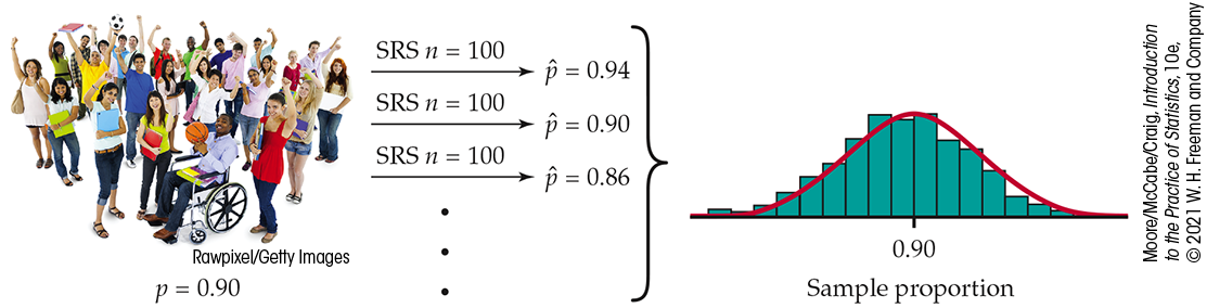
Figure 5.1 The
results of many SRSs have a regular pattern,
Example 5.3. Here
we draw SRSs of size
Of course, Student Monitor samples 1200 students, not just
100.
Figure 5.2
is parallel to Figure 5.1.
It shows the process of choosing 1000 SRSs, each of size 1200, from
a population in which the true proportion is
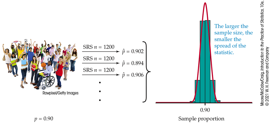
Figure 5.2 The distribution of the sample proportion for 1000 SRSs of size 1200 drawn from the same population as in Figure 5.1. The two histograms have the same x scale. The statistic from the larger sample is much less variable.
Strictly speaking, the sampling distribution is the ideal pattern that would emerge if we looked at all possible samples of size n (here, 100 or 1200) from our population. A distribution obtained from a fixed number of trials, like the 1000 trials in Figures 5.1 and 5.2, is only an approximation to the sampling distribution. We will see that probability theory, the mathematics of chance behavior, can sometimes describe sampling distributions exactly. The interpretation of a sampling distribution is the same, however, whether we obtain it by simulation or by the mathematics of probability.
Check-in
-
5.3 Poker winnings. Doug plays poker with the same group of friends once a week. At the end of the night, usually 2.5 to 3 hours later, he records how much he won or lost in an Excel spreadsheet. Does this collection of amounts represent an approximation to a sampling distribution of his average weekly winnings? Explain your answer.
We can use the tools of data analysis to describe any distribution. Let’s apply those tools to Figures 5.1 and 5.2.
-
Shape: The histograms look Normal. Figure 5.3 is a Normal quantile plot of the values of
-
Center: In both cases, the values of the sample proportion
-
Spread: The values of
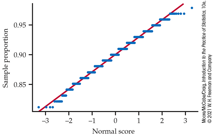
Figure 5.3 Normal quantile plot of the sample proportions in Figure 5.1. The distribution is close to Normal except for some clustering due to the fact that the sample proportions from a sample of size 100 can take only values that are a multiples of 0.01.
Although these results describe just two sets of simulations, they reflect facts that are true whenever we use random sampling.
Bias and variability
Our simulations show that a sample of size 1200 will almost always
give an estimate
Thinking about
Figures 5.1 and
5.2 helps us restate the
idea of bias when we use a statistic like
We can think of the true value of the parameter as the bull’s-eye on a target and of the sample statistic as an arrow fired at the bull’s-eye. Bias and variability describe what happens when an archer fires many arrows at the target. Bias means that the aim is off, and the sample values do not center about the population value. High variability means that sample values are widely scattered. In other words, there is a lack of precision, or consistency, among the sample values. Figure 5.4 shows this target illustration of the two types of error.
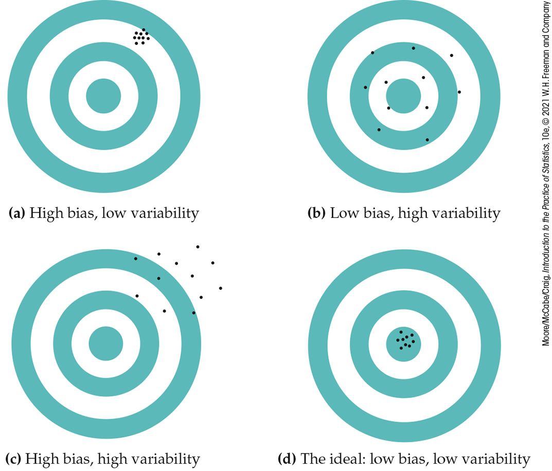
Figure 5.4 Bias and variability in shooting arrows at a target. Bias means the shots do not center around the bull’s-eye. Variability means that the shots are scattered.
Notice that low variability (repeated shots are close together) can accompany high bias (the arrows are consistently away from the bull’s-eye in one direction). And low bias (the arrows center on the bull’s-eye) can accompany high variability (repeated shots are widely scattered). A good sampling scheme, like a good archer, must have both low bias and low variability. Here’s how we ensure this.
In practice, Student Monitor takes only one random sample. We
don’t know how close to the truth the estimate from this one sample is
because we don’t know the value of the true parameter. But
large random samples almost always give an estimate that is close
to the truth.
Looking at the pattern of many samples when
Similarly, the Current Population Survey’s sample of about 60,000 households estimates the national unemployment rate very accurately. Of course, only probability samples carry this guarantee. Using a probability sampling design and taking care to deal with practical difficulties reduce bias in a sample.
The size of the sample then determines how close to the population truth the sample result is likely to fall. Results from a sample survey usually come with a margin of error that sets bounds on the size of the likely error.
Because the margin of error directly reflects the variability of the sample statistic, it is smaller for larger samples. In later chapters, we will describe the details of its calculation for many different statistics and how, when planning a survey or experiment, it is used to determine the sample size n.
Check-in
-
5.4 Bigger is better? Radio talk shows often report opinion polls based on thousands of listeners. These sample sizes are typically larger than those used in opinion polls that incorporate probability sampling. Does a larger sample size mean more trustworthy results? Explain your answer.
-
5.5 Effect of sample size on the sampling distribution. You are planning an opinion study and are considering taking an SRS of either 100 or 400 people. Explain how the sampling distributions of the population proportion p would differ in terms of center and spread for these two scenarios.
Sampling from large populations
Student Monitor’s sample of 1200 students is only about 1 out of every 9000 full-time undergraduate students in the United States. Does it matter whether we sample 1-in-1000 individuals in the population or 1-in-9000?
Why does the size of the population have little influence on the behavior of statistics from random samples? To see why this is plausible, imagine sampling harvested grain by thrusting a scoop into a lot of grain kernels. The scoop doesn’t know whether it is surrounded by a bag of grain or by an entire truckload. As long as the grain is well mixed (so that the scoop selects a random sample), the variability of the result depends only on the size of the scoop.
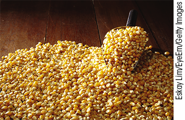
The fact that the variability of sample results is controlled by the size of the sample has important consequences for sampling design. An SRS of size 1200 from the 10.8 million undergraduates gives results as precise as an SRS of size 1200 from the roughly 85,000 inhabitants of San Francisco between the ages of 18 and 24. This is good news for designers of national samples but bad news for those who want accurate information about these citizens of San Francisco. If both use an SRS, both must use the same size sample to obtain equally trustworthy results.
Why randomize?
Why randomize? The act of randomizing guarantees that the results of analyzing our data are subject to the laws of probability. The behavior of statistics is described by a sampling distribution. The form of the distribution is known and, in many cases, is approximately Normal. Often, the center of the distribution lies at the true parameter value so that the notion that randomization eliminates bias is made more explicit. The spread of the distribution describes the variability of the statistic and can be made as small as we wish by choosing a large enough sample.
These facts are at the heart of formal statistical inference. The remainder of this chapter has much to say in more technical language about sampling distributions. Later chapters describe the way statistical conclusions are based on them. What any user of statistics must understand is that all the technical talk has its basis in a simple question: “What would happen if the sample or the experiment were repeated many times?” The reasoning applies not only to an SRS but also to the complex sampling designs actually used by opinion polls and other national sample surveys. The same conclusions hold as well for randomized experimental designs. The details vary with the design, but the basic facts are true whenever randomization is used to produce data.
Remember that proper statistical design is not the only aspect of a
good sample or experiment.
![]() The sampling distribution shows only how a statistic varies due to
the operation of chance in randomization. It reveals nothing about
possible bias due to undercoverage or nonresponse (page 185) in a sample or to lack of realism in an experiment.
The actual error in estimating a parameter by a statistic can be much
larger than the sampling distribution suggests. What is worse, there
is no way to say how large the added error is. The real world is less
orderly than statistics textbooks imply.
The sampling distribution shows only how a statistic varies due to
the operation of chance in randomization. It reveals nothing about
possible bias due to undercoverage or nonresponse (page 185) in a sample or to lack of realism in an experiment.
The actual error in estimating a parameter by a statistic can be much
larger than the sampling distribution suggests. What is worse, there
is no way to say how large the added error is. The real world is less
orderly than statistics textbooks imply.
In the next two sections, we will study the sampling distributions of two common statistics: the sample mean and the sample proportion. The focus will be on the important features of these distributions so that we can quickly describe and use them in the later chapters on statistical inference. We will see that, in each case, the sampling distribution depends on both the population and the way we collect the data from the population.
Section 5.1 SUMMARY
-
A number that describes a population is a parameter. A number that describes a sample, and is computed from the sample data, is a statistic.
-
The purpose of sampling or experimentation is usually statistical inference: using sample statistics to make statements about unknown parameters.
-
A statistic from a probability sample or a randomized experiment varies randomly from sample to sample. The sampling distribution of a statistic describes how the statistic varies in these repeated data productions. The sampling distribution answers the question “What would happen if we repeated the sample or experiment many times?” Formal statistical inference is based on the sampling distributions of statistics.
-
Simulation can be used to imitate the production of many random samples. If we calculate the statistic for each of these samples, their distribution approximates the statistic’s sampling distribution.
-
A statistic as an estimator of a parameter may suffer from bias or from large variability. Bias means that the center of the sampling distribution is not equal to the true value of the parameter. The variability of the statistic is described by the spread of its sampling distribution.
-
The spread of a statistic is usually reported by giving a margin of error for conclusions based on sample results. As the sample size increases, the margin of error decreases.
-
Properly chosen statistics from randomized data production designs have no bias resulting from the way the sample is selected or the way the experimental units are assigned to treatments. We can reduce the variability of the statistic by increasing the size of the sample.
-
As long as the population is at least 20 times larger than the sample size n, the size of the population has little influence on the variability of a statistic.
Section 5.1 EXERCISES
-
5.1 A change in the requirement rules? Thirty students from your liberal arts college are randomly selected to be on a committee to evaluate immediate changes in the quantitative competency requirement. There are 2600 students in your college. The current rules say that a statistics course is one of three options for a quantitative competency requirement. The proposed change would be to require a statistics course. Each of the committee members is asked to vote Yes or No on the new requirement.
Describe the population for this setting.
What is the parameter of interest?
What is the sample?
-
Describe the statistic and how it would be calculated.
-
Write a short summary based on your answers to parts (a) through (d) using this setting to explain population, sample, parameter, and statistic, as well as the relationships among these items.
-
5.2 What’s wrong? For each of the following statements, explain what is wrong and why.
A parameter describes a sample.
-
Bias and variability are two names for the same thing.
-
Large samples are always better than small samples.
-
A sampling distribution summarizes the values of a statistic for all possible samples from the same population.
-
5.3 Describe the population and the sample. For each of the following situations, describe the population and the sample.
-
A survey of 18,875 people aged 18 to 25 reported that 55.1% drank alcohol in the past month.
-
In a study of work stress, 250 restaurant workers were asked about the impact of work stress on their personal lives.
-
In a study of Monarch butterflies, 55 milkweed plants in a Yosemite Valley were randomly sampled. The average number of Monarch eggs per plant was 0.73.
-
-
5.4 Is it unbiased? A statistic has a sampling distribution that is somewhat skewed. The mean is 20.0, the median is 19.3, and the quartiles are 15.3 and 23.9.
-
If the true parameter value is 19.3, is the estimator unbiased?
-
If the true parameter value is 20.0, is the estimator unbiased?
-
If the true parameter value is 19.6, is the estimator unbiased?
-
Write a short summary of your results in parts (a), (b), and (c) and include a discussion of bias and unbiased estimators.
-
-
5.5 Constructing a sampling distribution. Refer to Example 5.1 (page 272). Suppose Student Monitor also reported that the median number of weekly hours per course spent outside of class was 2.5 hours.
-
Explain why we’d expect the population median to be less than the population mean in this setting by drawing the distribution of weekly hours per course spent outside of class for all undergraduates. This is called the population distribution.
-
Using Figure 5.2 (page 274) as a guide and your distribution from part (a), describe how to approximate the sampling distribution of the sample median in this setting.
-
-
5.6 Bias and variability. Figure 5.5 shows histograms of four sampling distributions of statistics intended to estimate the same parameter. Label each distribution relative to the others as high or low bias and as high or low variability.
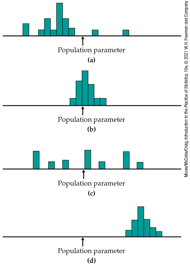
Figure 5.5 Determine which of these sampling distributions displays high or low bias and high or low variability, Exercise 5.6.
-
 5.7 Constructing sampling distributions.
The Probability applet simulates tossing a coin, with the
advantage that you can choose the true long-term proportion, or
probability, of a head. Suppose that we have a population in
which proportion
5.7 Constructing sampling distributions.
The Probability applet simulates tossing a coin, with the
advantage that you can choose the true long-term proportion, or
probability, of a head. Suppose that we have a population in
which proportion
-
Take 50 samples, recording the number of heads in each sample. Make a histogram of the 50 sample proportions (count of heads divided by 25). You are constructing the sampling distribution of this statistic.
-
Another population contains only 15% who plan to vote in the next election. Take 50 samples of size 25 from this population, record the number in each sample who approve, and make a histogram of the 50 sample proportions.
-
-
5.8 Comparing sampling distributions. Refer to the previous exercise.
-
How do the centers of your two histograms reflect the differing truths about the two populations?
-
Describe any differences in the shapes of the two histograms. Is one more skewed than the other?
-
Compare the spreads of the two histograms. For which population is there less sampling variability?
-
Suppose instead that the population proportions were 0.6 and 0.85, respectively. Describe how the sampling distributions of
-
-
5.9 Use the Simple Random Sample applet.
The Simple Random Sample applet can illustrate the idea
of a sampling distribution. Form a population labeled 1 to 100.
We will choose an SRS of 20 of these numbers. That is, in this
exercise, the numbers themselves are the population, not just
labels for 100 individuals. The mean of the whole numbers 1 to
100 is 50.5. This is the parameter, the mean of the population.
-
Use the applet to choose an SRS of size 20. Which 20 numbers were chosen? What is their mean? This is a statistic, the sample mean
-
Although the population and its mean 50.5 remain fixed, the sample mean changes as we take more samples. Take another SRS of size 20. (Use the “Reset” button to return to the original population before taking the second sample.) What are the 20 numbers in your sample? What is their mean? This is another value of
-
Take 23 more SRSs from this same population and record their means. You now have 25 values of the sample mean
-
-
5.10 Use the Simple Random Sample applet,
continued.
Refer to the previous exercise.
-
Suppose instead that a sample size of
-
Repeat the previous exercise using
-
Write a short paragraph about the effect of the sample size on the variability of a sampling distribution, using these simulations to illustrate the basic idea.
-
-
5.11 Sampling distributions and sample size. The software JMP includes some applets, one of which is called “Sampling Distribution of Sample Proportions.” This applet does sampling very quickly, especially if “Animate Illustration?” is set to No.
-
In Exercise 5.7, you obtained 50 draws of size
-
Keeping
-
Each sample size is four times larger than the previous one. For each adjacent pair compute the ratio of means and the ratio of standard deviations using the larger sample size in the denominator. Comment on what you find.
-
-
5.12 Twitter polls. Twitter provides the option for users to weigh in on questions posed by other Twitter users. A Twitter poll can remain open for a minimum of five minutes and maximum of one week after it is posted. Can you apply the ideas about populations and samples to these polls? Explain why or why not.