5.2 The Sampling Distribution of a Sample Mean
A variety of statistics are used to describe quantitative data. The sample mean, median, and standard deviation are all examples of statistics based on quantitative data. In the previous section, we learned that the general framework for constructing a sampling distribution is the same for all statistics and that we can approximate a sampling distribution through simulation. In this section, we will concentrate on the sample mean and study its sampling distribution using both simulation and statistical theory. Because sample means are just averages of observations, they are among the most frequently used statistics.
Suppose that you plan to survey 1000 undergraduates enrolled in
four-year U.S. universities about their sleeping habits when at school.
The sampling distribution of the average hours of sleep per night
describes what this average would be if many simple random samples of
1000 students were drawn from the population of students in the United
States. In other words, it gives you an idea of what you are likely to
see from your survey. It tells you whether you should expect this
average to be near the population mean and whether its margin of error
is roughly

Before constructing this distribution, however, we need to consider another set of probability distributions that plays a role in statistical inference. Imagine choosing only one individual at random from the population and measuring a quantity. The values obtained from repeated draws of one individual from the population have a probability distribution that is called the population distribution.
Example 5.4 Total sleep time of college students.
A study of sleep quality and academic performance describes the distribution of sleep duration among students as approximately Normal, with a mean of 7.13 hours and standard deviation of 1.67 hours.4 Suppose that we select a college student at random and obtain their average sleep time. This result is a random variable X because, prior to the random sampling, we don’t know the sleep time. We do know, however, that in repeated sampling, X will have the same N(7.13, 1.67) distribution that describes the pattern of sleep time in the entire population. We call N(7.13, 1.67) the population distribution. This is the context in which we first met distributions, as density curves that provide models for the overall pattern of data.
In this example, the population of all college students actually exists so that we can, in principle, draw an SRS of students from it. Sometimes, our population of interest does not actually exist. For example, suppose that we are interested in studying final-exam scores in a statistics course, and we have the scores of the 103 students who took the course last semester. For the purposes of statistical inference, we might want to consider these 103 students as part of a hypothetical population of similar students who would take this course. In this sense, these 103 students represent not only themselves but also a larger population of similar students. The key idea is to think of the observations that you have as coming from a population with a probability distribution.
Check-in
-
5.6 Time spent using apps on a smartphone. In “How to Win Gen Z on Mobile,” App Annie reports that Gen Z smartphone users worldwide average 92.5 hours per month using the top 25 non-gaming apps.5
-
State the population that this report describes and the statistic.
-
Sketch what you think this population distribution would look like, making sure to specify its mean and median.
-
Now that we have made the distinction between the population
distributions and sampling distributions, we can proceed with an
in-depth study of the sampling distribution of a sample mean
Example 5.5 Sample means are approximately Normal.
![]()
Figure 5.6(a)
displays the distribution of student visit lengths (in minutes) to a
statistics help room at a large midwestern university. Students
visiting the help room were asked to sign in upon arrival and then
sign out when leaving. During the school year, there were 1838 visits
to the help room but only 1264 recorded visit lengths because many
visiting students forgot to sign out.6
The distribution is strongly skewed to the right, with a maximum visit
length of 485 minutes. The population mean is
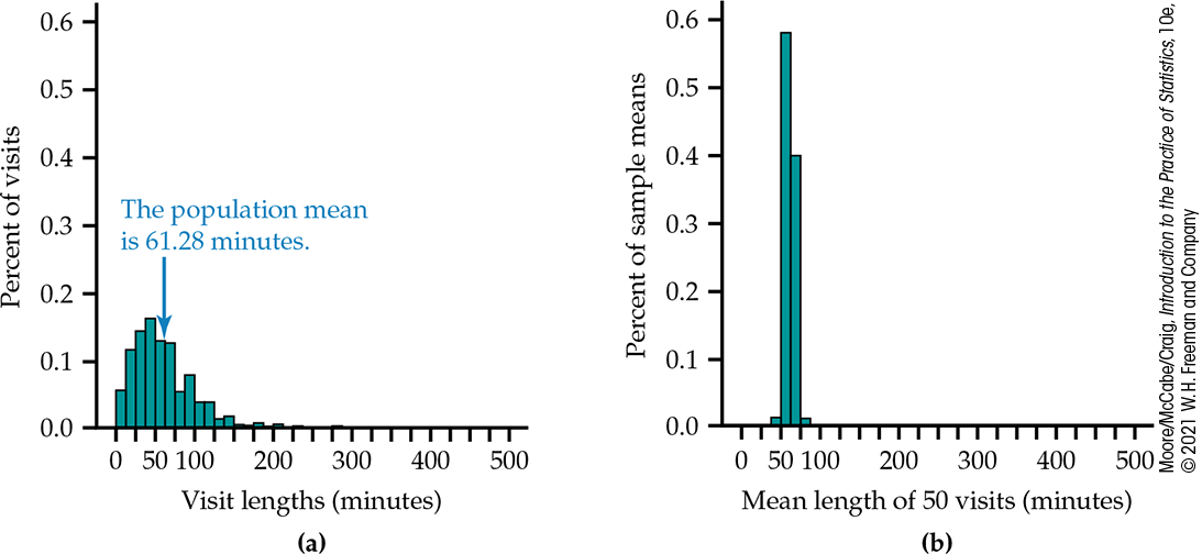
Figure 5.6 (a) The
distribution of 1264 visit lengths to a statistics help room
during the school year,
Example 5.5. (b) The
distribution of the sample means
| 5 | 6 | 14 | 15 | 20 | 20 | 20 | 28 | 30 | 30 |
| 30 | 30 | 31 | 33 | 35 | 40 | 41 | 41 | 41 | 50 |
| 50 | 55 | 55 | 55 | 55 | 55 | 60 | 60 | 60 | 65 |
| 65 | 65 | 66 | 67 | 75 | 75 | 80 | 85 | 85 | 86 |
| 90 | 90 | 98 | 99 | 110 | 122 | 142 | 150 | 160 | 165 |
![]()
TABLE 5.1 contains the
lengths of a random sample of 50 visits from this population. The mean
of these 50 visits is
Figure 5.6(b) illustrates
several striking facts about the sampling distribution of a sample
mean. First, the sample means are much less spread out than the
individual visit lengths. Second, the sample means appears centered
around population mean
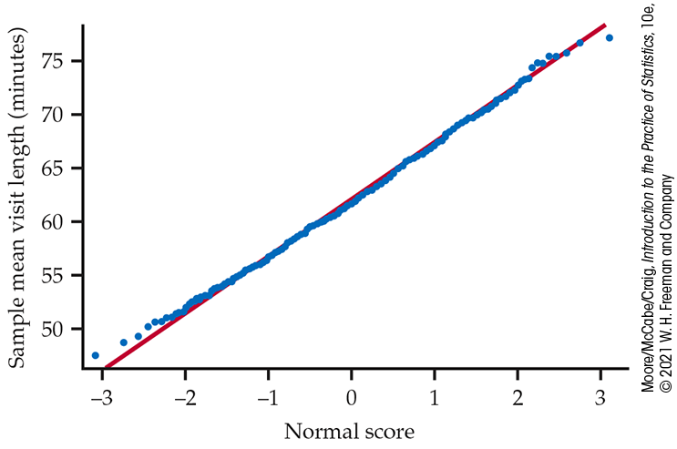
Figure 5.7 Normal quantile plot of the 500 sample means in Figure 5.6(b). The distribution is close to Normal.
These three facts contribute heavily to the popularity of sample means in statistical inference. Let’s now study each of them more carefully using statistical theory.
The mean and standard deviation of
x ¯
The sample mean
The design used to produce the data.
-
The sample size n.
The population distribution.
Suppose we select an SRS of size n from a population and
measure a variable X on each individual in the sample. The
n measurements are values of n random variables
The sample mean of an SRS of size n is
If the population has mean
That is,
the mean of
Because the observations are independent, the addition rule for variances also applies:
With n in the denominator, the variability of
How precisely does a sample mean
Because the standard deviation of
Example 5.6 Standard deviations for sample means of visit lengths.
The standard deviation of the population of visit lengths in
Figure 5.6(a) is
Averaging over more visits reduces the variability and makes it more
likely that
Check-in
-
5.7 Find the mean and the standard deviation of the sampling distribution. Compute the mean and standard deviation of the sampling distribution of the sample mean when you plan to take an SRS of size 25 from a population with mean 215 and standard deviation 10.
-
5.8 The effect of increasing the sample size. In the setting of the previous exercise, repeat the calculations for a sample size of 100. Explain the effect of the sample size increase on the mean and standard deviation of the sampling distribution.
Before discussing the third fact, we have one comment on terminology.
To maintain the distinction between parameters and statistics, the
term “standard error” is sometimes used for the standard deviation of
a statistic. Thus, the standard deviation of
The central limit theorem
![]()
We have described the center and spread of the probability
distribution of a sample mean
Most population distributions are non-Normal. Yet
Figures 5.6(b) and
5.7 show that means of
samples of size 50 from a strongly skewed population are close to
Normal. Clearly, there must be something more we can say about the
sampling distribution of
One of the most famous facts of probability theory says that, for
large sample sizes, the distribution of
Example 5.7 How close will the sample mean be to the population mean?
With the Normal distribution to work with, we can better describe
how precisely a random sample of 50 visits estimates the mean length
of all visits to the statistics help room. The population standard
deviation for the 1264 visits in the population of
Figure 5.6(a) is
If a margin of error of 11.8 minutes is not considered precise enough,
we must consider a larger sample size to reduce the standard deviation
of
Example 5.8 Reducing the
standard deviation of
x ¯
In the setting of
Example 5.7, if we
want to reduce the standard deviation of
For samples of size 200, about 95% of the sample means will be
within twice 2.96, or 5.9 minutes, of the population mean
The standard deviation computed in
Example 5.8 is actually
too large. This is due to the fact that the population size,
![]() When
When
Thus, for samples of size 200, about 95% of the sample means will be
within twice 2.72, or 5.4 minutes, of the population mean
Check-in
-
5.9 Use the 68–95–99.7 rule. You take an SRS of size 25 from a population with mean 215 and standard deviation 10. According to the central limit theorem, what is the approximate sampling distribution of the sample mean? Use the 95 part of the 68–95–99.7 rule to determine the margin of error.
-
5.10 Increasing the sample size. Refer to the previous Check-in question. Suppose that you increase the sample size to 225. Use the 95 part of the 68–95–99.7 rule to determine the margin of error. By what factor is the margin of error reduced?
The main point of
Examples 5.7 and
5.8 is to demonstrate
that the central limit theorem allows us to use Normal probability
calculations to answer questions about sample means even when the
population distribution is not Normal.
Example 5.8, however,
reminds us that if the population is very spread out, the
The central limit theorem can be used when “n is large.” How
large n has to be for
Example 5.9 The central limit theorem in action.
Figure 5.8
shows the central limit theorem in action for another very
non-Normal population.
Figure 5.8(a) displays the
density curve of a single observation from the population. The
distribution is strongly right-skewed, and the most probable
outcomes are near 0. The mean
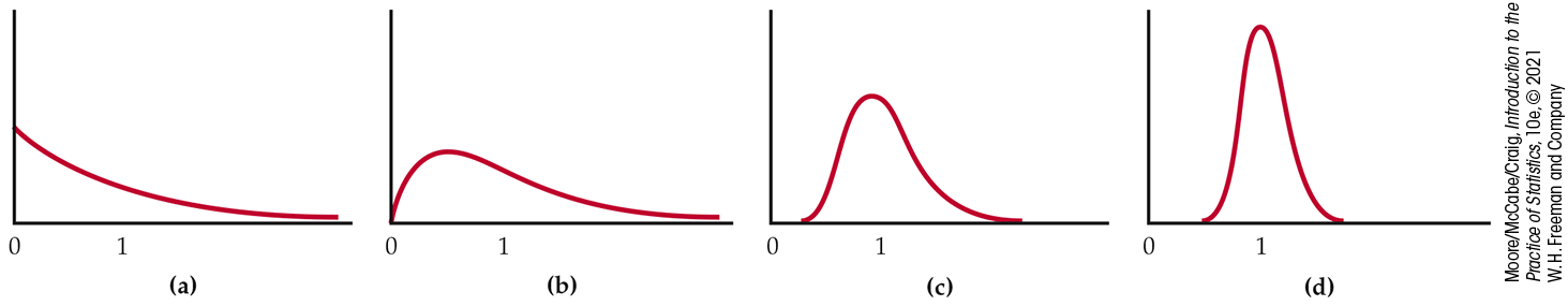
Figure 5.8 The
central limit theorem in action: the sampling distribution of
sample means from a strongly non-Normal population becomes more
Normal as the sample size increases,
Example 5.9. The
distribution of (a) 1 observation; (b)
Figures 5.8(b), (c), and
(d) are the density curves of the sample means of 2, 10, and 25
observations from this population. As n increases, the shape
becomes more Normal. The mean remains at
![]() You can also use the Central Limit Theorem applet to study the
sampling distribution of
You can also use the Central Limit Theorem applet to study the
sampling distribution of
Example 5.10 Using the Central Limit Theorem applet.
In Example 5.9, we
considered sample sizes of
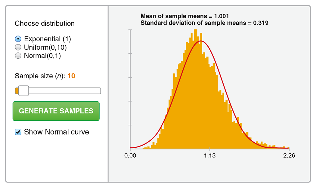
Figure 5.9 Screenshot
of the Central Limit Theorem applet for the exponential
distribution when
Try using the applet for the other sample sizes in Example 5.9. You should get histograms shaped like the density curves shown in Figure 5.8. You can also consider other sample sizes by sliding n from 1 to 100. As you increase n, the shape of the histogram moves closer to the Normal curve that is based on the central limit theorem.
Check-in
-
 5.11 Use the Central Limit Theorem applet.
Let’s consider the uniform distribution between 0 and 10. For
this distribution, all intervals of the same length between 0
and 10 are equally likely. This distribution has a mean of 5 and
standard deviation of 2.89.
5.11 Use the Central Limit Theorem applet.
Let’s consider the uniform distribution between 0 and 10. For
this distribution, all intervals of the same length between 0
and 10 are equally likely. This distribution has a mean of 5 and
standard deviation of 2.89.
-
Approximate the population distribution by setting
-
What are your estimates of the population mean and population standard deviation based on the 10,000 SRSs? Are these population estimates close to the true values?
-
Describe the shape of the histogram and compare it with the Normal curve.
-
-
5.12 Use the Central Limit Theorem applet
again.
Refer to the previous Check-in question. In the setting of
Example 5.9, let’s
approximate the sampling distribution for samples of size
-
For each sample size, compute the mean and standard deviation of
-
For each sample size, use the applet to approximate the sampling distribution. Report the estimated mean and standard deviation. Are they close to the true values calculated in part (a)?
-
For each sample size, compare the shape of the sampling distribution with the Normal curve based on the central limit theorem.
-
For this population distribution, what sample size do you think is needed to make you feel comfortable using the central limit theorem to approximate the sampling distribution of
-
Now that we know that the sampling distribution of the sample mean
Example 5.11 Time between snaps.

Snapchat has more than 200 million daily users sending well over 3
billion snaps a day.7
Suppose that the time X between snaps you receive is governed
by the exponential distribution with mean
The central limit theorem says that the sample mean time
The sampling distribution of
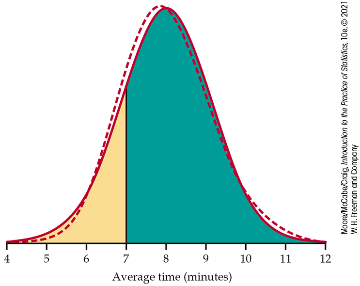
Figure 5.10 The exact distribution (dashed) and the Normal approximation from the central limit theorem (solid) for the average time between snaps received, Example 5.11.
The probability we want is
The exactly correct probability is the area under the dashed density curve in the figure. It is 0.8094. The central limit theorem Normal approximation is off by only about 0.0012.
We can also use this sampling distribution to talk about the total time between the 1st and 51st snap received.
Example 5.12 Convert the results to the total time.
There are 50 time intervals between the 1st and 51st snap. According to the central limit theorem calculations in Example 5.11,
We know that the sample mean is the total time divided by 50, so the
event
Check-in
-
5.13 Find a probability. Refer to Example 5.11. Find the probability that the mean time between snaps is less than 8 minutes. The exact probability is 0.5188. Compare your answer with the exact one.
Figure 5.11
summarizes the facts about the sampling distribution of
-
Take many random samples of size n from a population with mean
-
Find the sample mean
-
Collect all the
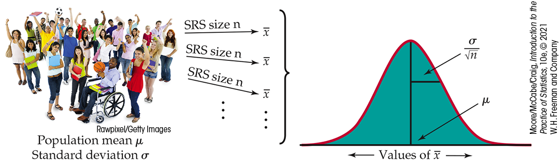
Figure 5.11 The
sampling distribution of a sample mean
The sampling distribution of
A few more facts related to the sampling distribution of
x ¯
Even though the central limit theorem is the big fact of probability
theory in this section, there are several additional facts related to
our investigations of the sampling distribution of
The fact that the sample mean of an SRS from a Normal population has a
Normal distribution is a special case of a more general fact:
any linear combination of independent Normal random variables is
also Normally distributed.
That is, if X and Y are independent Normal random
variables and a and b are any fixed numbers,
Example 5.13 Getting to and from campus.
You live off campus and take the shuttle provided by your apartment complex to and from campus. Your time on the shuttle, in minutes, varies from day to day. The time going to campus X has the N(20, 4) distribution, and the time returning from campus Y varies according to the N(18, 8) distribution. If they vary independently, what is the probability that you will be on the shuttle for less time going to campus?
The difference in times
Because
Although, on average, it takes longer to go to campus than return, the trip to campus will take less time on roughly two of every five days.
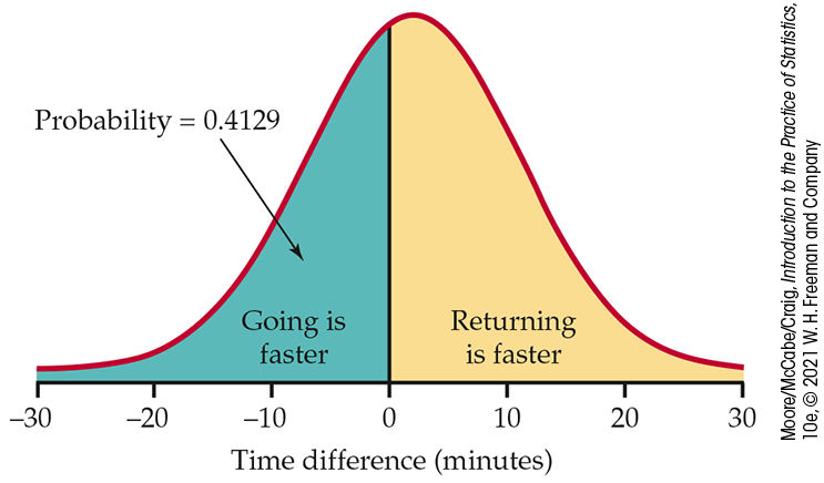
Figure 5.12 The
Normal probability calculation,
Example 5.13. The
difference in times going to campus and returning from campus
The second useful fact is that more general versions of the central limit theorem say that the distribution of a sum or an average of many small random quantities is close to Normal. This is true even if the quantities are not independent (as long as they are not too highly correlated) and even if they have different distributions (as long as no single random quantity is so large that it dominates the others). These more general versions of the central limit theorem suggest why the Normal distributions are common models for observed data. Any variable that is a sum of many small random influences will have approximately a Normal distribution.
Finally, the central limit theorem also applies to discrete random variables. An average of discrete random variables will never result in a continuous sampling distribution, but the Normal distribution often serves as a good approximation. In the next section, we will discuss the sampling distribution and Normal approximation for counts and proportions. This Normal approximation is just an example of the central limit theorem applied to these discrete random variables.
Example 5.14 Weibull density curves.
Figure 5.13 shows the density curves of three members of the Weibull family. Each describes a different type of distribution for the time to failure of a product.
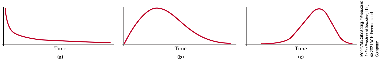
Figure 5.13 Density curves for three members of the Weibull family of distributions, Example 5.14. The curves model (a) infant mortality, (b) early failure, and (c) old-age wear-out.
-
Figure 5.13(a) is a model for infant mortality. This describes products that often fail immediately, prior to delivery to the customer. However, if the product does not fail right away, it will likely last a long time. For products like this, a manufacturer might test them and ship only the ones that do not fail immediately.
-
Figure 5.13(b) is a model for early failure. These products do not fail immediately, but many fail early in their lives after they are in the hands of customers. This is disastrous, and the product or the process that makes it must be changed at once.
-
Figure 5.13(c) is a model for old-age wear-out. Most of these products fail only when they begin to wear out, and then many fail at about the same age.
A manufacturer certainly wants to know to which of these classes a
new product belongs. To find out, engineers operate a random sample
of products until they fail. From the failure time data, we can
estimate the parameter (called the “shape parameter”) that
distinguishes among the three Weibull distributions in
Figure 5.13. The shape
parameter has no simple definition like that of a population
proportion or mean, and it cannot be estimated by a simple statistic
such as
Two things save the situation. First, statistical theory provides
general approaches for finding good estimates of any parameter.
These general methods not only tell us how to use
Section 5.2 SUMMARY
-
The population distribution of a variable X is the distribution of its values for all members of the population. This distribution and the sample size n affect the distribution of
-
The sample mean
-
The sample mean
-
The standard deviation of
-
The central limit theorem states that, for large n, the sampling distribution of
-
Linear combinations of independent Normal random variables have Normal distributions. In particular, if the population has a Normal distribution, so does
Section 5.2 EXERCISES
-
5.13 What’s wrong? For each of the following statements, explain what is wrong and why.
-
If the population standard deviation is 20, then the standard deviation of
-
When taking SRSs from a population, larger sample sizes will result in larger standard deviations of
-
For an SRS from a population, both the mean and the standard deviation of
-
The larger the population, the bigger the sample size n needs to be for a desired standard deviation of
-
-
5.14 What’s wrong? For each of the following statements, explain what is wrong and why.
-
The central limit theorem states that for large n, the population mean
-
For large n, the distribution of observed values will be approximately Normal.
-
For sufficiently large n, the 68–95–99.7 rule says that
-
Refer to Figure 5.13. For
-
-
5.15 Generating a sampling distribution. Let’s illustrate the idea of a sampling distribution in the case of a very small sample from a very small population. The population is the 10 scholarship players currently on your women’s basketball team. For convenience, the 10 players have been labeled with the integers 0 to 9. For each player, the total amount of time spent (in minutes) on Twitter during the past week is recorded in the following table.
Player 0 1 2 3 4 5 6 7 8 9 Time (min) 118 24 89 85 74 135 116 107 60 99 The parameter of interest is the average amount of time on Twitter. The sample is an SRS of size
-
Find the mean for the 10 players in the population. This is the population mean
-
Use Table B to draw an SRS of size 3 from this population. (Note: You may sample the same player’s time more than once.) Write down the three times in your sample and calculate the sample mean
-
Repeat this process nine more times, using different parts of Table B. Make a histogram of the 10 values of
-
Is the center of your histogram close to
-
-
5.16 Sleep duration of college students. In Example 5.4, the daily sleep duration among college students was approximately Normally distributed with mean
-
What is the standard deviation for the average time?
-
Use the 95 part of the 68–95–99.7 rule to describe the variability of this sample mean.
-
What is the probability that your average will be below 6.9 hours?
-
-
5.17 Determining sample size. Refer to the previous exercise. You want to use a sample size such that about 95% of the averages fall within
-
Based on your answer to part (b) in Exercise 5.16, should the sample size be larger or smaller than 60? Explain.
-
What standard deviation of
-
Using the standard deviation you calculated in part (b), determine the number of students you need to sample.
-
-
5.18 Length of a movie on Netflix. Flixable reports that Netflix’s U.S. catalog contains almost 4000 movies.9 You are interested in determining the average length of these movies. Previous studies have suggested the standard deviation for this population is 34 minutes.
-
What is the standard deviation of the average length if you take an SRS of 25 movies from this population?
-
How many movies would you need to sample if you wanted the standard deviation of
-
-
5.19 Bottling an energy drink. A bottling company uses a filling machine to fill cans with an energy drink. The cans are supposed to contain 250 milliliters (ml) each. The machine, however, has some variability, so the standard deviation of the volume is
-
5.20 Average movie length on Netflix. Refer to Exercise 5.18. Suppose that the true mean movie length is 98.6 minutes, and you plan to take an SRS of
-
Explain why it may be reasonable to assume that the average
-
Sketch the approximate Normal curve for the sample mean, making sure to specify its mean and standard deviation.
-
What is the probability that your sample mean will differ from the population mean by more than 2 minutes?
-
-
5.21 Can volumes. Averages are less variable than individual observations. It is reasonable to assume that the can volumes in Exercise 5.19 vary according to a Normal distribution. In that case, the mean
-
Make a sketch of the Normal curve for a single can. Add the Normal curve for the mean of an SRS of five cans on the same sketch.
-
What is the probability that the volume of a single randomly chosen can differs from the target value by 0.1 ml or more?
-
What is the probability that the mean volume of an SRS of five cans differs from the target value by 0.1 ml or more?
-
-
5.22 Number of friends on Facebook. In Australia, young people aged 18 to 29 have an average of 394 Facebook friends.10 This population distribution takes only integer values, so it is certainly not Normal. It is also highly skewed to the right. Suppose that
-
For your sample, what are the mean and standard deviation of
-
Use the central limit theorem to find the probability that the average number of friends for an SRS of 70 Facebook users is greater than 425.
-
What are the mean and standard deviation of the total number of friends in your sample?
-
What is the probability that the total number of friends among your sample of 70 Facebook users is greater than 29,750?
-
-
5.23 Cholesterol levels of teenagers. A study of the health of teenagers plans to measure the blood cholesterol level of an SRS of 13- to 16-year-olds. The researchers will report the mean
-
Explain to someone who knows no statistics what it means to say that
-
The sample result
-
-
5.24 Grades in a math course. Indiana University posts the grade distributions for its courses online.11 In one spring semester, students in Math 118 received 16.1% A’s, 34.3% B’s, 29.2% C’s, 9.6% D’s, and 9.8% F’s.
-
Using the common scale
-
Math 118 is a large enough course that we can take the grades of an SRS of 25 students and not worry about the finite population correction factor. If
-
What is the probability that a randomly chosen Math 118 student gets a B or better,
-
What is the approximate probability that the grade point average for 25 randomly chosen Math 118 students is B or better,
-
Explain why the probabilities in parts (c) and (d) are so different.
-
-
5.25 Weights of airline passengers. In 2019, the Federal Aviation Administration (FAA) updated its standard average passenger weight to be based on data from U.S. government health agency surveys.12 It specified this average weight, which includes clothing, as 189 pounds in the summer (195 in the winter). These health agency surveys can also be used to determine the standard deviation, which we’ll assume is 47 pounds. Weights are not Normally distributed, especially when the population includes both men and women, but they are not very non-Normal. A commuter plane carries 25 passengers. What is the approximate probability that, in the winter, the total weight of the passengers exceeds 5225 pounds? (Hint: To apply the central limit theorem, restate the problem in terms of the mean weight.)
-
 5.26 Investments in two funds. Jennifer invests
her money in a portfolio that consists of 65% Fidelity 500 Index
Fund and 35% Fidelity Tax-Free Bond Fund. Suppose that, in the
long run, the annual real return X on the Index Fund has
mean 10% and standard deviation 12%, the annual real return
Y on the Bond Fund has mean 5% and standard deviation 3%,
and the correlation between X and Y is
5.26 Investments in two funds. Jennifer invests
her money in a portfolio that consists of 65% Fidelity 500 Index
Fund and 35% Fidelity Tax-Free Bond Fund. Suppose that, in the
long run, the annual real return X on the Index Fund has
mean 10% and standard deviation 12%, the annual real return
Y on the Bond Fund has mean 5% and standard deviation 3%,
and the correlation between X and Y is
-
The return on Jennifer’s portfolio is
-
The distribution of returns is typically roughly symmetric but with more extreme high and low observations than a Normal distribution. The average return over a number of years, however, is close to Normal. If Jennifer holds her portfolio for 20 years, what is the approximate probability that her average return is greater than 5%?
-
The calculation you just made is not overly helpful because Jennifer isn’t really concerned about the mean return
-