4.4 Means and Variances of Random Variables
The probability histograms and density curves that picture the probability distributions of random variables resemble our earlier pictures of distributions of data. In describing data, we moved from graphs to numerical measures such as means and standard deviations. Now we will make the same move to expand our descriptions of the distributions of random variables. We can speak of the mean winnings in a game of chance or the standard deviation of the randomly varying number of calls a travel agency receives in an hour. In this section, we will learn more about how to compute these descriptive measures and about the laws they obey.
The mean of a random variable
In Chapter 1 (page 26), we learned that the mean
If we think of a random process as corresponding to the population, then the mean of the random variable is a characteristic of this population. Here is an example.
Example 4.33 The Tri-State Pick 3 lottery.
Most states and Canadian provinces have government-sponsored lotteries. Here is a simple lottery wager, from the Tri-State Pick 3 game that New Hampshire shares with Maine and Vermont. You choose a three-digit number, 000 to 999. The state chooses a three-digit winning number at random and pays you $500 if your number is chosen.
Because there are 1000 three-digit numbers, you have probability 1/1000 of winning. Taking X to be the amount your ticket pays you, the probability distribution of X is
| Payoff X | $0 | $500 |
| Probability | 0.999 | 0.001 |
The random process consists of drawing a three-digit number. The population consists of the numbers 000 to 999. Each of these possible outcomes is equally likely. In the setting of sampling in Chapter 3 (page 181), we can view the random process as selecting an SRS of size 1 from the population. The random variable X is $500 if the selected number is equal to the one that you chose and is $0 if it is not.
What is your average payoff from many tickets? The ordinary average of the two possible outcomes $0 and $500 is $250, but that makes no sense as the average because $500 is much less likely than $0. In the long run, you receive $500 once in every 1000 tickets and $0 on the remaining 999 of 1000 tickets. The long-run average payoff is
or 50 cents. That number is the mean of the random variable X. (Tickets cost $1, so in the long run, the state keeps half the money you wager.)
If you play Tri-State Pick 3 several times, we would—as usual—call the
mean of the actual amounts you win
Check-in
-
4.16 Find the mean of the probability distribution. You toss a fair coin. If the outcome is heads, you win $20; if the outcome is tails, you win nothing. Let X be the amount that you win in a single toss of a coin. Find the probability distribution of this random variable and its mean.
Just as probabilities are an idealized description of long-run
proportions, the mean of a probability distribution describes the
long-run average outcome. We can’t call this mean
To remind ourselves that we are talking about the mean of X, we
often write
The mean of any discrete random variable is found just as in Example 4.33. It is an average of the possible outcomes—but it is a weighted average in which each outcome is weighted by its probability. Because the probabilities add to 1, we have total weight 1 to distribute among the outcomes. An outcome that occurs half the time has probability one-half and gets one-half the weight in calculating the mean. Here is the general definition.
Example 4.34 The mean of equally likely first digits.
If first digits in a set of data all have the same probability, the probability distribution of the first digit X is then
| First digit X | 1 | 2 | 3 | 4 | 5 | 6 | 7 | 8 | 9 |
| Probability |
|
|
|
|
|
|
|
|
|
The mean of this distribution is
Suppose that the random digits in Example 4.34 had a different probability distribution. In Example 4.15 (page 215), we described Benford’s law as a probability distribution that describes first digits of numbers in many real situations. Let’s calculate the mean for Benford’s law.
Example 4.35 The mean of first digits that follow Benford’s law.
Here is the distribution of the first digit for data that follow Benford’s law. We use the letter V for this random variable to distinguish it from the one that we studied in Example 4.34. The distribution of V is
| First digit V | 1 | 2 | 3 | 4 | 5 | 6 | 7 | 8 | 9 |
| Probability | 0.301 | 0.176 | 0.125 | 0.097 | 0.079 | 0.067 | 0.058 | 0.051 | 0.046 |
The mean of V is
The mean reflects the greater probability of smaller first digits under Benford’s law than when first digits 1 to 9 are equally likely.
Figure 4.13 locates the means of X and V on the two probability histograms. Because the discrete uniform distribution of Figure 4.13(a) is symmetric, the mean lies at the center of symmetry. We can’t precisely locate the mean of the right-skewed distribution of Figure 4.13(b) by eye; calculation is needed.
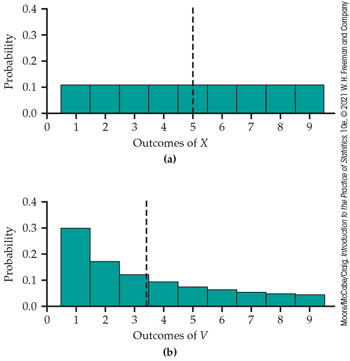
Figure 4.13 Locating the mean of a discrete random variable on the probability histogram for (a) digits between 1 and 9 chosen at random; (b) digits between 1 and 9 chosen from records that obey Benford’s law.
What about continuous random variables? The probability distribution of a continuous random variable X is described by a density curve. Chapter 1 (page 49) showed how to find the mean of the distribution: it is the point at which the area under the density curve would balance if it were made out of solid material. The mean lies at the center of symmetric density curves such as the Normal curves. Exact calculation of the mean of a distribution with a skewed density curve requires advanced mathematics.12 The idea that the mean is the balance point of the distribution applies to discrete random variables as well, but in the discrete case, we have a formula that gives us this point.
Statistical estimation and the law of large numbers
We would like to estimate the mean height
Statistics obtained from probability samples are random variables because their values vary in repeated sampling. The sampling distributions of statistics are just the probability distributions of these random variables.
It seems reasonable to use
If
The behavior of
Example 4.36 Heights of young women.
The distribution of the heights of all young women is close to the
Normal distribution with mean 64.5 inches and standard deviation 2.5
inches. Suppose that
Figure 4.14
shows the behavior of the mean height
This is the second point on the line in the graph.
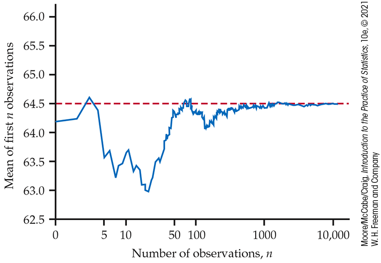
Figure 4.14 The law of large numbers in action, Example 4.36. As we take more observations, the sample mean always approaches the mean of the population.
At first, the graph shows that the mean of the sample changes as we
take more observations. Eventually, however, the mean of the
observations gets close to the population mean
Check-in
-
 4.17 Use the Law of Large Numbers applet.
The Law of Large Numbers applet animates a graph like
Figure 4.14
for rolling dice. Use it to better understand the law of large
numbers by making a similar graph.
4.17 Use the Law of Large Numbers applet.
The Law of Large Numbers applet animates a graph like
Figure 4.14
for rolling dice. Use it to better understand the law of large
numbers by making a similar graph.
The mean
Thinking about the law of large numbers
The law of large numbers says broadly that the average results of many independent observations are stable and predictable. The gamblers in a casino may win or lose, but the casino will win in the long run because the law of large numbers says what the average outcome of many thousands of bets will be. An insurance company deciding how much to charge for life insurance and a fast-food restaurant deciding how many beef patties to prepare also rely on the fact that averaging over many individuals produces a stable result. It is worth the effort to think a bit more closely about such an important fact.
The “law of small numbers”
Both the rules of probability and the law of large numbers describe the regular behavior of chance phenomena in the long run. Psychologists have discovered that our intuitive understanding of randomness is quite different from the true laws of chance.13 For example, most people believe in an incorrect “law of small numbers.” That is, we expect even short sequences of random events to show the kind of average behavior that in fact appears only in the long run.
Some teachers of statistics begin a course by asking students to toss a coin 50 times and bring the sequence of heads and tails to the next class. The teacher then announces which students just wrote down a random-looking sequence rather than actually tossing a coin. The faked tosses don’t have enough “runs” of consecutive heads or consecutive tails. Runs of the same outcome don’t look random to us but are, in fact, common. For example, the probability of a run of three or more consecutive heads or tails in just 10 tosses is greater than 0.8.14 The runs of consecutive heads or consecutive tails that appear in real coin tossing (and that are predicted by the mathematics of probability) seem surprising to us. Because we don’t expect to see long runs, we may conclude that the coin tosses are not independent or that some influence is disturbing the random behavior of the coin.
Example 4.37 The “hot hand” in basketball.
Belief in the law of small numbers influences behavior. If a basketball player makes several consecutive shots, both the fans and her teammates believe that she has a “hot hand” and is more likely to make the next shot. This is doubtful.
Careful study suggests that runs of baskets made or missed are no more frequent in basketball than would be expected if each shot were independent of the player’s previous shots. Baskets made or missed are just like heads and tails in tossing a coin. (Of course, some players make 30% of their shots in the long run and others make 50%, so a coin-toss model for basketball must allow coins with different probabilities of a head.) Our perception of hot or cold streaks simply shows that we don’t perceive random behavior very well.15
![]() Our intuition doesn’t do a good job of distinguishing random
behavior from systematic influences. This is also true when we
look at data.
We need statistical inference to supplement exploratory analysis of
data because probability calculations can help verify that what we
see in the data is more than a random pattern.
Our intuition doesn’t do a good job of distinguishing random
behavior from systematic influences. This is also true when we
look at data.
We need statistical inference to supplement exploratory analysis of
data because probability calculations can help verify that what we
see in the data is more than a random pattern.
How large is a large number?
The law of large numbers says that the actual mean outcome of many
trials gets close to the distribution mean
Example 4.38 Laws of large numbers for gambling.
Serious gamblers sometimes follow a system of betting in which the
amount bet on each play depends on the outcome of previous plays.
You might, for example, double your bet on each spin of the
roulette wheel until you win—or, of course, until your fortune is
exhausted. Such a system tries to take advantage of the fact that
you have a memory even though the roulette wheel does not. Can you
beat the odds with a system based on the outcomes of past plays?
No. Mathematicians have established a stronger version of the law
of large numbers that says that, if you do not have an infinite
fortune to gamble with, your long-run average winnings
Example 4.39 Another law of large numbers.
You are in charge of a process that manufactures video screens for
computer monitors. Your equipment measures the tension on the
metal mesh that lies behind each screen and is critical to its
image quality. You want to estimate the mean tension
Rules for means
We occasionally need to apply a linear transformation,
Example 4.40 Paint flaws on refrigerators.
You are studying flaws in the painted finish of refrigerators made
by your firm. Dimples and paint sags are two kinds of surface flaw.
Not all refrigerators have the same number of dimples: many have
none, some have one, some two, and so on. You ask for the average
number of imperfections on a refrigerator. The inspectors report
finding an average of 0.7 dimples and 1.4 sags per refrigerator. How
many total imperfections of both kinds (on the average) are there on
a refrigerator? That’s easy: if the average number of dimples is 0.7
and the average number of sags is 1.4, then counting both gives an
average of
In more formal language, the number of dimples on a refrigerator is a
random variable X that varies as we inspect one refrigerator
after another. We know only that the mean number of dimples is
That’s an important rule for how means of random variables behave. Here’s another example describing a different rule.
Example 4.41 Crickets.
The crickets living in a field have mean length of 1.2 inches. What
is the mean in centimeters? There are 2.54 centimeters in an inch,
so the length of a cricket in centimeters is 2.54 times its length
in inches. If we multiply every observation by 2.54, we also
multiply their average by 2.54. The mean in centimeters must be
The point of these examples is that means behave like averages. Here are the rules written in more formal language.
Example 4.42 How many courses?

In Exercise 4.35 (page 233), you described the probability distribution of the number of courses taken in the fall by students at a small liberal arts college. Here is the distribution:
| Courses in the fall | 1 | 2 | 3 | 4 | 5 | 6 |
| Probability | 0.06 | 0.06 | 0.12 | 0.20 | 0.41 | 0.15 |
For the spring semester, the distribution is a little different:
| Courses in the spring | 1 | 2 | 3 | 4 | 5 | 6 |
| Probability | 0.06 | 0.08 | 0.15 | 0.25 | 0.34 | 0.12 |
For a randomly selected student, let X be the number of courses taken in the fall semester and let Y be the number of courses taken in the spring semester. The means of these random variables are
The mean course load for the fall is 4.29 courses, and the mean
course load for the spring is 4.09 courses. We assume that these
distributions apply to students who earned credit for courses taken
in the fall and the spring semesters. The mean of the total number
of courses taken for the academic year is
Note that it is not possible for a student to take 8.38 courses in an academic year. This number is the mean of the probability distribution.
Example 4.43 What about credit hours?
In the previous exercise, we examined the number of courses taken in
the fall and in the spring at a small liberal arts college. Suppose
that we were interested in the total number of credit hours earned
for the academic year. We assume that for each course taken at this
college, three credit hours are earned. Let T be the mean of
the distribution of the total number of credit hours earned for the
academic year. What is the mean of the distribution of T? To
find the answer, we can use Rule 1 with
The mean of the distribution of the total number of credit hours earned is 25.14.
Check-in
-
4.18 Find
-
4.19 Find
The variance of a random variable
The mean is a measure of the center of a distribution. A basic
numerical description requires, in addition, a measure of the spread
or variability of the distribution. The variance and the standard
deviation are the measures of spread that accompany the choice of the
mean to measure center. Just as for the mean, we need a distinct
symbol to distinguish the variance of a random variable from the
variance
The definition of the variance
For discrete random variables, the average we use is a weighted average in which each outcome is weighted by its probability. Calculating this weighted average is straightforward. For continuous random variables, however, advanced mathematics is needed. Here is the formula for the discrete case.
Example 4.44 Find the mean, the variance, and the standard deviation.
In Example 4.42, we saw that the distribution of the number X of fall courses taken by students at a small liberal arts college is
| Courses in the fall | 1 | 2 | 3 | 4 | 5 | 6 |
| Probability | 0.06 | 0.06 | 0.12 | 0.20 | 0.41 | 0.15 |
We can find the mean and variance of X by arranging the
calculation in the form of a table. Both
|
|
|
|
|
| 1 | 0.06 | 0.06 |
|
| 2 | 0.06 | 0.12 |
|
| 3 | 0.12 | 0.36 |
|
| 4 | 0.20 | 0.80 |
|
| 5 | 0.41 | 2.05 |
|
| 6 | 0.15 | 0.90 |
|
|
|
|
||
We see that
Check-in
-
4.20 Find the variance and the standard deviation. The random variable X has the following probability distribution:
Value of X 0 4 Probability 0.2 0.8 Find the variance
Rules for variances and standard deviations
What are the facts for variances that parallel Rules 1, 2, and 3 for
means?
![]() The mean of a sum of random variables is always the sum of their
means, but this addition rule is true for variances only in special
situations.
The following example explains why.
The mean of a sum of random variables is always the sum of their
means, but this addition rule is true for variances only in special
situations.
The following example explains why.
Example 4.45 Family finances.
Take X to be the percent of a family’s after-tax income that
is spent, and take Y to be the percent that is saved. When
X increases, Y decreases by the same amount. Though
X and Y may vary widely from year to year, their sum
If random variables are independent, this kind of association between their values is ruled out, and their variances do add. Two random variables X and Y are independent if knowing that any event involving X alone did or did not occur tells us nothing about the occurrence of any event involving Y alone.
Probability models often assume independence when the random variables describe outcomes that appear unrelated to each other. You should ask in each instance whether the assumption of independence seems reasonable.
When random variables are not independent, the variance of their sum
depends on the correlation between them as well as on their
individual variances. In
Chapter 2, we met the
correlation r between two observed variables measured on the
same individuals. We defined the correlation r as an average of
the products of the standardized x and y observations.
The correlation between two random variables is defined in the same
way. We won’t give the details; it is enough to know that the
correlation between two random variables has the same basic properties
as the correlation r calculated from data. We use
Example 4.46 Correlation for family finances.
Refer to the family finances setting in
Example 4.45. If X is the percent of a family’s after-tax income that is
spent and Y is the percent that is saved, then
With the correlation at hand, we can state the rules for manipulating variances.
![]() Because a variance is the average of squared deviations from the
mean, multiplying X by a constant b multiplies
Because a variance is the average of squared deviations from the
mean, multiplying X by a constant b multiplies
As with data, we prefer the standard deviation to the variance as a
measure of the variability of a random variable.
![]() Rule 2 for variances implies that standard deviations of
independent random variables do
not
add. To combine standard deviations, use the rules for
variances.
For example, the standard deviations of 2X and
Rule 2 for variances implies that standard deviations of
independent random variables do
not
add. To combine standard deviations, use the rules for
variances.
For example, the standard deviations of 2X and
Example 4.47 Payoff in the Tri-State Pick 3 lottery.
The payoff X of a $1 ticket in the Tri-State Pick 3 game is $500 with probability 1/1000 and 0 the rest of the time. Here is the combined calculation of mean and variance:
|
|
|
|
|
| 0 | 0.999 | 0 |
|
| 500 | 0.001 | 0.5 |
|
|
|
|
||
The mean payoff is 50 cents. The standard deviation is
If you buy a Pick 3 ticket, your winnings are
Example 4.48 Winnings in the Tri-State Pick 3 lottery.
The winnings are
That is, you lose an average of a half dollar on a ticket. The rules
for variances remind us that the variance and standard deviation of
the winnings
Example 4.49 Express the winnings in cents.
Using the information from the previous example, let’s express the
winnings in cents. The winnings in cents are 100X, and the
ticket cost is 100 cents. Our winnings in cents is the random
variable
Suppose now that you buy a $1 ticket on each of two different days.
The payoffs X and Y on the two tickets are independent
because separate drawings are held each day. Your total payoff is
Example 4.50 Two tickets.
The mean for the payoff for the two tickets is
Because X and Y are independent, the variance of
The standard deviation of the total payoff is
This is not the same as the sum of the individual standard
deviations, which is
Suppose that we buy 20 lottery tickets. The same rules for means and
variances of independent random variables works for any number of
random variables. Therefore, the mean for 20 tickets is
When we add random variables that are correlated, we need to use the correlation for the calculation of the variance but not for the calculation of the mean. Here is an example.
Example 4.51 Utility bills.
Consider a household where the monthly bill for natural gas averages
$125, with a standard deviation of $75, while the monthly bill for
electricity averages $174, with a standard deviation of 41. The
correlation between the two bills is
Let’s compute the mean and standard deviation of the sum of the
natural-gas bill and the electricity bill. We let X stand for
the natural-gas bill and Y stand for the electricity bill.
Then the total is
To find the standard deviation, we first find the variance and then take the square root to determine the standard deviation. From the general addition rule for variances of random variables,
Therefore, the standard deviation is
The total of the natural-gas bill and the electricity bill has mean $299 and standard deviation $63.
The negative correlation in Example 4.51 is due to the fact that, in this household, natural gas is used for heating, and electricity is used for air-conditioning. So, when it is warm, the electricity charges are high, and the natural-gas charges are low. When it is cool, the reverse is true. This causes the standard deviation of the sum to be less than it would be if the two bills were uncorrelated (see Exercise 4.68, page 252).
There are situations where we need to combine several of our rules to find means and standard deviations. Here is an example.
Example 4.52 Calcium intake.
To get enough calcium for optimal bone health, tablets containing calcium are often recommended to supplement the calcium in the diet. One study designed to evaluate the effectiveness of a supplement followed a group of young people for seven years. Each subject was assigned to take either a tablet containing 1000 milligrams of calcium per day (mg/d) or a placebo tablet that was identical except that it had no calcium.16 A major problem with studies like this one is compliance: subjects do not always take the treatments assigned to them.
In this study, the compliance rate declined to about 47% toward the end of the seven-year period. The standard deviation of compliance was 22%. Calcium from the diet averaged 850 mg/d, with a standard deviation of 330 mg/d. The correlation between compliance and dietary intake was 0.68. Let’s find the mean and standard deviation for the total calcium intake. We let S stand for the intake from the supplement and D stand for the intake from the diet.
We start with the intake from the supplement. Because the compliance is 47% and the amount in each tablet is 1000 mg, the mean for S is
Because the standard deviation of the compliance is 22%, the variance of S is
The standard deviation is
Be sure to verify which rules for means and variances are used in these calculations.
We can now find the mean and standard deviation for the total intake. The mean is
the variance is
and the standard deviation is
The mean of the total calcium intake is 1320 mg/d, and the standard deviation is 506 mg/d.
The correlation in this example illustrates an unfortunate fact about compliance and having an adequate diet. Some of the subjects in this study have diets that provide an adequate amount of calcium, while others do not. The positive correlation between compliance and dietary intake tells us that those who have relatively high dietary intakes are more likely to take the assigned supplements. On the other hand, subjects with relatively low dietary intakes, the ones who need the supplement the most, are less likely to take the assigned supplements.
Section 4.4 SUMMARY
-
The probability distribution of a random variable X, like a distribution of data, has a mean
-
The law of large numbers says that the average of the values of X observed in many trials must approach
-
The mean
-
The variance
-
The standard deviation
-
The mean and variance of a continuous random variable can be computed from the density curve, but to do so requires more advanced mathematics.
-
The means and variances of random variables obey the following rules. If a and b are fixed numbers, then
-
If X and Y are any two random variables having correlation
-
If X and Y are independent, then
-
To find the standard deviation, take the square root of the variance.
Section 4.4 EXERCISES
-
4.56 Different kinds of means. Explain the difference between the mean of a random variable and the mean of a sample.
-
4.57 Find the mean of the random variable. A random variable X has the following distribution:
X 0 1 Probability 0.1 0.2 0.4 0.3 Find the mean for this random variable. Show your work.
-
4.58 Servings of fruits and vegetables. The following table gives the distribution of the number of servings of fruits and vegetables consumed per day in a population:
Number of servings X 0 1 2 3 4 5 Probability 0.4 0.1 0.1 0.2 0.1 0.1 Find the mean for this random variable.
-
4.59 Explain what happens when the sample size gets large. Consider the following scenarios: (1) You take a sample of two observations on a random variable and compute the sample mean, (2) you take a sample of 100 observations on the same random variable and compute the sample mean, (3) you take a sample of 1000 observations on the same random variable and compute the sample mean. Explain in simple language how close you expect the sample mean to be to the mean of the random variable as you move from Scenario 1 to Scenario 2 to Scenario 3.
-
4.60 What’s wrong? In each of the following scenarios, there is something wrong. Describe what is wrong and give a reason for your answer.
-
If you toss a fair coin three times and get heads all three times, then the probability of getting a tail on the next toss is much greater than one-half.
-
If you multiply a random variable by 10, then the mean is multiplied by 10 and the variance is multiplied by 10.
-
When finding the mean of the sum of two random variables, you need to know the correlation between them.
-
-
4.61 Find some means. Suppose that X is a random variable with mean 20 and standard deviation 2. Also suppose that Y is a random variable with mean 40 and standard deviation 7. Assume that the correlation between X and Y is zero. Find the mean of the random variable Z for each of the following cases. Be sure to show your work.
-
-
4.62 Mean of the distribution for the number of aces. In Exercise 4.47 (page 234) you examined the probability distribution for the number of aces when you are dealt two cards in the game Texas hold ’em. Let X represent the number of aces in a randomly selected deal of two cards in this game. Here is the probability distribution for the random variable X:
Value of X 0 1 2 Probability 0.8507 0.1448 0.0045 Find
-
4.63 Find the variance and the standard deviation. A random variable X has the following distribution:
X 0 1 Probability 0.1 0.2 0.4 0.3 Find the variance and the standard deviation for this random variable. Show your work.
-
4.64 Standard deviation of the number of aces. Refer to Exercise 4.62. Find the standard deviation of the number of aces.
-
4.65 Find some variances and standard deviations. Suppose that X is a random variable with mean 20 and standard deviation 3. Also suppose that Y is a random variable with mean 60 and standard deviation 2. Assume that the correlation between X and Y is zero. Find the variance and the standard deviation of the random variable Z for each of the following cases. Be sure to show your work.
-
-
4.66 Standard deviation for fruits and vegetables. Refer to Exercise 4.58. Find the variance and the standard deviation for the distribution of the number of servings of fruits and vegetables.
-
 4.67 What happens if the correlation is not zero?
Suppose that X is a random variable with mean 20 and
standard deviation 3. Also suppose that Y is a random
variable with mean 60 and standard deviation 2. Assume that the
correlation between X and Y is 0.4. Find the
variance and the standard deviation of the random
variable Z for each of the following cases. Be sure to
show your work.
4.67 What happens if the correlation is not zero?
Suppose that X is a random variable with mean 20 and
standard deviation 3. Also suppose that Y is a random
variable with mean 60 and standard deviation 2. Assume that the
correlation between X and Y is 0.4. Find the
variance and the standard deviation of the random
variable Z for each of the following cases. Be sure to
show your work.
-
-
4.68 Suppose that the correlation is zero. Refer to Example 4.51 (page 248).
-
Recompute the standard deviation for the total of the natural-gas bill and the electricity bill, assuming that the correlation is zero.
-
Is this standard deviation larger or smaller than the standard deviation computed in Example 4.51? Explain why.
-
-
4.69 Find the mean of the sum. Figure 4.12 (page 235) displays the density curve of the sum
-
The mean of a continuous random variable is the balance point of its density curve. Use this fact to find the mean of Y from Figure 4.12.
-
Use the same fact to find the means of
-
-
4.70 Calcium supplements and calcium in the diet. Refer to Example 4.52 (page 249). Suppose that people who have high intakes of calcium in their diets are more compliant than those who have low intakes. What effect would this have on the calculation of the standard deviation for the total calcium intake? Explain your answer.
-
4.71 Toss a four-sided die twice.
Role-playing games like Dungeons & Dragons use many
different types of dice. Suppose that a four-sided die has faces
marked 1, 2, 3, and 4. The intelligence of a character is
determined by rolling this die twice and adding 1 to the sum of
the spots. The faces are equally likely, and the two rolls are
independent. What is the average (mean) intelligence for such
characters? How spread out are their intelligences, as measured
by the standard deviation of the distribution?
-
4.72 Means and variances of sums. The rules for means and variances allow you to find the mean and variance of a sum of random variables without first finding the distribution of the sum, which is usually much harder to do.
-
A single toss of a balanced coin has either 0 or 1 head, each with probability 1/2. What are the mean and standard deviation of the number of heads?
-
Toss a coin four times. Use the rules for means and variances to find the mean and standard deviation of the total number of heads.
-
Example 4.27 (page 227) finds the distribution of the number of heads in four tosses. Find the mean and standard deviation from this distribution. Your results in parts (b) and (c) should agree.
-
-
4.73 What happens when the correlation is 1?
We know that variances add if the random variables involved are
uncorrelated
-
4.74 Will you assume independence? In which of the following games of chance would you be willing to assume independence of X and Y in making a probability model? Explain your answer in each case.
-
In blackjack, you are dealt two cards and examine the total points X on the cards (face cards count 10 points). You can choose to be dealt another card and compete based on the total points Y on all three cards.
-
In craps, the betting is based on successive rolls of two dice. X is the sum of the faces on the first roll, and Y the sum of the faces on the next roll.
-
-
4.75 Transform the distribution of heights from centimeters to inches. A report of the National Center for Health Statistics says that the heights of 20-year-old men have mean 176.8 centimeters (cm) and standard deviation 7.2 cm. There are 2.54 centimeters in an inch. What are the mean and standard deviation in inches?
-
4.76 Fire insurance. An insurance company looks at the records for millions of homeowners and sees that the mean loss from fire in a year is
-
4.77 Mean and standard deviation for 5 policies and for 20 policies. In fact, the insurance company in the previous exercise sees that in the entire population of homeowners, the mean loss from fire is