6.4 Inference as a Decision in Chapter 6 Introduction to Inference

6.4 Inference as a Decision

We have presented tests of significance as methods for assessing the strength of evidence against the null hypothesis. This assessment is made by the P-value, which is a probability computed under the assumption that H0 is true. The alternative hypothesis (the statement we seek evidence for) enters the test only to help us see what outcomes count against the null hypothesis.

There is, however, another way to think about these issues. Sometimes, we are really concerned about making a decision or choosing an action based on our evaluation of the data. Acceptance sampling is one such circumstance. Suppose a producer of ball bearings and a skateboard manufacturer agree that each shipment of bearings shall meet certain quality standards. When a lot of bearings arrives, the manufacturer chooses a sample of bearings to be inspected. On the basis of the sample outcome, the manufacturer will either accept or reject the lot. Let’s examine how the idea of inference as a decision changes the reasoning used in tests of significance.

Two types of error

Tests of significance concentrate on H0, the null hypothesis. If a decision is called for, however, there is no reason to single out H0. There are simply two hypotheses, and we must choose one and reject the other. It is convenient to call the two hypotheses H0 and Ha, but H0 no longer has the special status (the statement we try to find evidence against) that it had in tests of significance. In our acceptance sampling example, we must decide between

H0:the lot of bearings meets standardsHa:the lot does not meet standards

on the basis of a sample of bearings.

We hope that our decision will be correct, but sometimes it will be wrong. There are two types of incorrect decisions. We can accept a bad lot of bearings, or we can reject a good lot. Accepting a bad lot injures the consumer, while rejecting a good lot hurts the producer. To help distinguish these two types of error, we give them specific names.

These possibilities are summarized in Figure 6.16 for the acceptance sampling example. If H0 is true, our decision is either correct or a Type I error. If Ha is true, our decision is either correct or a Type II error. Only one error is possible at one time.

A matrix of error types. — Figure 6.16 The two types of error in the acceptance sampling example.

Significance tests with fixed-level α give a rule for making decisions because the test either rejects H0 or fails to reject it. If we adopt the decision-making way of thought, failing to reject H0 means choosing H0. We can then describe the performance of a significance test by the probabilities of Type I and Type II errors. This is summarized in Figure 6.17.

Error probabilities

Any rule for making decisions is assessed in terms of the probabilities of the two types of error. This is in keeping with the idea that statistical inference is based on probability. We cannot (short of inspecting the whole lot) guarantee that good lots of bearings will never be rejected and bad lots will never be accepted. But by random sampling and the laws of probability, we can say what the probabilities of both kinds of error are.

Example 6.29 Outer diameter of a skateboard bearing.

The mean outer diameter of a skateboard bearing is supposed to be 22.000 millimeters (mm). The outer diameters vary Normally, with standard deviation σ=0.010 mm. When a lot of the bearings arrives, the skateboard manufacturer takes an SRS of five bearings from the lot and measures their outer diameters. The manufacturer rejects the bearings if the sample mean diameter is significantly different from 22 mm at the 5% significance level.

This is a test of the hypotheses

H0: μ=22Ha: μ≠22

To carry out the test, the manufacturer computes the z statistic:

z=x¯-220.01/5

and rejects H0 if

z≤−1.96 or z≥1.96

A Type I error is to reject H0 when in fact μ=22.

What about Type II errors? Because there are many values of μ in Ha, we will concentrate on one value of μ. There is, however, a Type II error probability for each μ in Ha. For this example, we’ll assume that the producer and the manufacturer agree that a lot of bearings with mean 0.015 mm away from the desired mean 22.000 should be rejected. So a particular Type II error is to choose H0 when in fact μ=22.015.

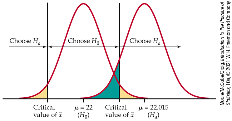
Figure 6.18 shows how the two probabilities of error are obtained from the two sampling distributions of x¯, for μ=22 and for μ=22.015. When μ=22, H0 is true and to choose Ha (reject H0) is a Type I error. When μ=22.015, choosing H0 is a Type II error. We will now calculate these error probabilities.

Two side-by-side, overlapping normal distribution curves. — Figure 6.18 The two error probabilities, Example 6.29. The probability of a Type I error (yellow area) is the probability of choosing Ha: μ≠22 when in fact μ=22. The probability of a Type II error (blue area) is the probability of choosing H0 when in fact μ=22.015.

Two side-by-side normal distribution curves are plotted on the same horizontal axis, overlapping each other. The left curve has mean mu equals 22, representing H sub 0. The right curve has mean mu equals 22.015, representing H sub a. Critical values of x bar are marked under the left tails of each curve. The area under the curves to the left of their critical values is shaded. The right tail of the left curve overlaps the critical value and mean of the right curve. The area under the right tail of the left curve, to the right of the other curve’s critical value is shaded. For values between the two critical values, choose H sub 0. For values right of the right curve’s critical value, choose H sub a. For values left of the left curve’s critical value, choose H sub a.

The probability of a Type I error is the probability of rejecting H0 when it is really true. In Example 6.29, this is the probability that |z|≥1.96 when μ=22. But this is exactly the significance level of the test. The critical value 1.96 was chosen to make this probability 0.05, so we do not have to compute it again. The definition of “significant at level 0.05” is that sample outcomes this extreme will occur with probability 0.05 when H0 is true.

The probability of a Type II error for the particular alternative μ=22.015 in Example 6.29 is the probability that we choose H0 (fail to reject H0) when μ has this alternative value. The complement of this probability is the probability that we choose Ha (reject H0) when Ha is true. This probability also has a special name.

High power is desirable as it implies that the probability of a Type II error is small. Similar to choosing the sample size for a desired margin of error of a confidence interval (page 340), one can determine the sample size needed for a desired power at a particular alternative. We discuss the use of software to do these calculations in the next chapter.

For now, we can see from Figure 6.18 that the probability of a Type II error requires specifying the rejection region in terms of x¯ and then standardizing the endpoints using μ=22.015 (see Exercise 6.84). The probability of a Type II error turns out to be 0.08, which means the power of this test is 1−0.08, or 0.92. Rejecting a lot (choosing Ha) over 9 out of 10 times in this setting gives the manufacturer confidence that the ball bearings will not have too large a diameter.

Applet The Statistical Power applet can also be used to compute the error probabilities. For this calculation, we’d enter the null (μ=22) and alternative (μ≠22) hypotheses, the sample size (n=5), the standard deviation (σ=0.01), and the significance level (α=0.05). We’d also set alt μ to 22.015.

The distinction between tests of significance and tests as rules for deciding between two hypotheses does not lie in the calculations but in the reasoning that motivates the calculations. In a test of significance, we focus on a single hypothesis (H0) and a single probability (the P-value). The goal is to measure the strength of the sample evidence against H0. Calculations of power are done to check the sensitivity of the test. If we cannot reject H0, we conclude only that there is not sufficient evidence against H0, not that H0 is actually true.

If the same inference problem is thought of as a decision problem, we focus on two hypotheses and give a rule for deciding between them based on the sample evidence. Therefore, we must focus equally on two probabilities, the probabilities of the two types of error. We must choose one hypothesis and cannot abstain on grounds of insufficient evidence.

The common practice of testing hypotheses

Clearly distinguishing the two ways of thinking is helpful for understanding. In practice, the two approaches often merge. We continued to call one of the hypotheses in a decision problem H0. The common practice of testing hypotheses mixes the reasoning of significance tests and decision rules as follows:

State H0 and Ha just as in a test of significance.
Think of the problem as a decision problem, so that the probabilities of Type I and Type II errors are relevant.
Because of Step 1, Type I errors are more serious. So choose an α (significance level) and consider only tests with probability of a Type I error no greater than α.
Among these tests, select one that makes the probability of a Type II error as small as possible (that is, power as large as possible).

Testing hypotheses may seem to be a hybrid approach. It was, historically, the effective beginning of decision-oriented ideas in statistics. An impressive mathematical theory of hypothesis testing was developed between 1928 and 1938 by Jerzy Neyman and Egon Pearson. The decision-making approach came later (1940s). Because decision theory in its pure form leaves you with two error probabilities and no simple rule on how to balance them, it has been used less often than either tests of significance or tests of hypotheses. Decision ideas have been applied in testing problems mainly by way of the Neyman–Pearson hypothesis-testing theory. That theory asks you first to choose α, and the influence of Fisher has often led users of hypothesis testing comfortably back to α=0.05 or α=0.01. Fisher, who was exceedingly argumentative, violently attacked the Neyman–Pearson decision-oriented ideas, and the argument still continues.

Section 6.4 SUMMARY

An alternative to significance testing regards H0 and Ha as two statements of equal status that we must decide between. This decision theory point of view regards statistical inference in general as giving rules for making decisions in the presence of uncertainty. Acceptance sampling is one example of this approach.
In the case of testing H0 versus Ha, decision analysis chooses a decision rule on the basis of the probabilities of two types of error. A Type I error occurs if Ha is chosen (H0 is rejected) when it is in fact H0 true. A Type II error occurs if H0 is chosen (fail to reject H0) when in fact Ha is true.
The power of a test measures its ability to detect an alternative hypothesis. The power to detect a specific alternative is calculated as the probability that the test will choose Ha (reject H0) when that alternative is true.
In a fixed-level α significance test, the significance level α is the probability of a Type I error, and the power to detect a specific alternative is 1 minus the probability of a Type II error for that alternative.

Now that you have completed this section, you will be able to:

Describe the two types of possible errors when performing a test that focuses on deciding between two hypotheses. Review Example 6.29 (page 376) and try Exercise 6.79.
Describe the two types of possible errors when performing a test of significance. Review Example 6.29 (page 376) and try Exercise 6.81.
Define what is meant by the power of a test. Review Example 6.29 (page 376) and try Exercise 6.83.
Relate the two errors to the significance level and power of the test. Review Example 6.29 (page 376) and try Exercise 6.85.

Section 6.4 EXERCISES

6.78 A role as a statistical consultant. You are the statistical expert for a graduate student planning her PhD research. After you carefully present the mechanics of significance testing, she suggests using α=0.20 for the study because she would be more likely to obtain statistically significant results, and she thinks that she really needs to find significant results to graduate. Explain in terms of testing errors why this would not be a good use of statistical methods.
6.79 What are the Type I and Type II errors? A smartphone manufacturer gets its phone batteries from one supplier. For each shipment, a random sample of n=6 batteries are tested to ensure that the shipment complies with specifications, such as capacity and discharge curve levels.
1. Specify the hypotheses the manufacturer must decide between.
2. Describe what a Type I and a Type II error would be, based on your specification of hypotheses in part (a).

NAEP 6.80 Choose the appropriate distribution. You must decide which of two discrete distributions a random variable X has. We will call the distributions p0 and p1. Here are the probabilities assigned to the values x of X:

x	0	1	2	3	4	5	6
p0	0.0	0.1	0.1	0.1	0.4	0.2	0.1
p1	0.2	0.4	0.2	0.1	0.1	0.0	0.0

You have a single observation on X and wish to choose between

H0:p0 is correctHa:p1 is correct

One possible decision procedure is to reject H0 only if X≤2.

Find the probability of a Type I error—that is, the probability that you choose Ha (reject H0) when p0 is the correct distribution.
Find the probability of a Type II error.

6.81 Percent energy from added sugars: Type I and Type II errors. A test of significance was performed in Example 6.15 (page 357).
1. Describe the Type I and Type II errors in this example.
2. Based on the conclusion, which type of error might have occurred? Explain your answer.
6.82 Choose the appropriate distribution, continued. Refer to Exercise 6.80. Another possible decision procedure is to reject H0 if X≤3.
1. Find the probabilities of a Type I and Type II error under this decision procedure.
2. Which decision procedure, X≤2 or X≤3, do you prefer? Explain your answer.
6.83 What is the power of the test? A study is run to test H0: μ=50 using the two-sided alternative and the α=0.01 significance level. For each of the following settings, give the power of the test when μ=55.
1. The probability of a Type II error when μ=55 is 0.43.
2. The probability of a Type II error when μ=55 is 0.19.
3. The probability of a Type II error when μ=45 is 0.08.
6.84 Computing the power in the ball bearing study. Recall Example 6.29. Let’s run through the steps needed to obtain the power of 0.92 when μ=22.015.
1. Given that we reject H0 if z≤−1.96 or z≥1.96 and
  
  z=x¯-220.01/5,
  
  for what values of x¯ do we reject H0?
2. Now assuming x¯~N(22.015,0.01/5), verify that the probability that an x¯ falls in the region specified by part (a) is 0.92.
6.85 Power for a different alternative. For the ball bearing example (page 376), the power is 0.92 when μ=22.015.
1. Would the power for the alternative μ=22.030 be larger than, smaller than, or equal to 0.92? Sketch a plot like Figure 6.18 to explain your answer.
2. Use the Statistical Power applet to verify your answer in part (a).
6.86 More on choosing the appropriate distribution. Refer to Exercise 6.80. Suppose that instead of a single observation X, you plan to obtain n observations and use the decision rule to reject H0 when x¯≤k.
1. What are the means of x¯ under p0 and p1?
2. Based on your answers in part (a), what would be a good choice for k? Explain your answer.
6.87 Computer-assisted career guidance systems. A wide variety of computer-assisted career guidance systems have been developed over the past decade. These programs use factors such as student interests, aptitude, skills, personality, and family history to recommend a career path. For simplicity, suppose that a program recommends that a high school graduate either go to college or join the workforce.
1. What are the two hypotheses and the two types of error that the program can make?
2. The program can be adjusted to decrease one error probability at the cost of an increase in the other error probability. Which error probability would you choose to make smaller, and why? (This is a matter of judgment. There is no single correct answer.)
6.88 Effect of changing the alternative μ on power. The Statistical Power applet can be used to study power. Open the applet and set the null hypothesis to μ=0, the alternative to μ>0, the sample size to n=10, the standard deviation to σ=1, the significance level to α=0.05, and the alternative μ to 1. What is the power? Repeat for alternative μ equal to 0.1, 0.2, 0.3, 0.4, 0.5, 0.6, 0.7, 0.8, 0.9. Make a table or graph giving μ and the power. What do you conclude?
6.89 Other changes and the effect on power. Refer to the previous exercise. For each of the following changes, explain what happens to the power for each alternative μ.
1. Change to the two-sided alternative.
2. Decrease σ to 0.5.
3. Increase n from 10 to 30.
6.90 Make a recommendation. Your manager has asked you to review a research proposal that includes a section on sample size justification. A careful reading of this section indicates that the power is 18% for detecting an effect that would be considered important. Write a short report for your manager explaining what this means and make a recommendation on whether or not this study should be run as designed.