6.1 Estimating with Confidence
The SAT and ACT are two standardized tests used to assess readiness for college study. Until recently, one of these two tests was required by most colleges for admission. Even though many universities are now considering test-optional admissions, the tests are still used by states and universities for comparison and benchmarking purposes.
The SAT consists of two sections, one for mathematics (SATM) and one for critical reading and writing (SATW), and an optional essay. Possible scores on each section range from 200 to 800, for a total range of 400 to 1600. Since 1995, section scores have been recentered so that the mean is approximately 500 with a standard deviation of 100 in a large “standardized group.” This scale has been maintained so that scores have a constant interpretation over time.
Example 6.3 Estimating the mean SATM score for seniors in California.

Suppose that you want to estimate the mean SATM score for the 489,650
high school seniors in California.2
You know better than to trust data from the students who choose to
take the SAT. Only about 56% of California students typically take the
SAT.3
These self-selected students are planning to attend college and are
not representative of all California seniors. At considerable effort
and expense, you give the test to an SRS of 500 California high school
seniors. The mean score for your sample is
The sample mean
But how reliable is this estimate? A second sample of 500 students would surely not give a sample mean of 505 again. Unbiasedness says only that there is no systematic tendency to underestimate or overestimate the truth. Could we plausibly get a sample mean of 493 and a sample mean of 517 in repeated samples? An estimate without an indication of its variability is of little value.
Statistical confidence
The unbiasedness of an estimator concerns the center of its sampling
distribution, but questions about variation are answered by looking at
its spread. The central limit theorem says that if the entire
population of SATM scores has mean
Now we are ready to proceed. Consider this line of thought, which is illustrated in Figure 6.2:
-
The 68–95–99.7 rule says that the probability is about 0.95 that
-
To say that
-
So about 95% of all samples will contain the true
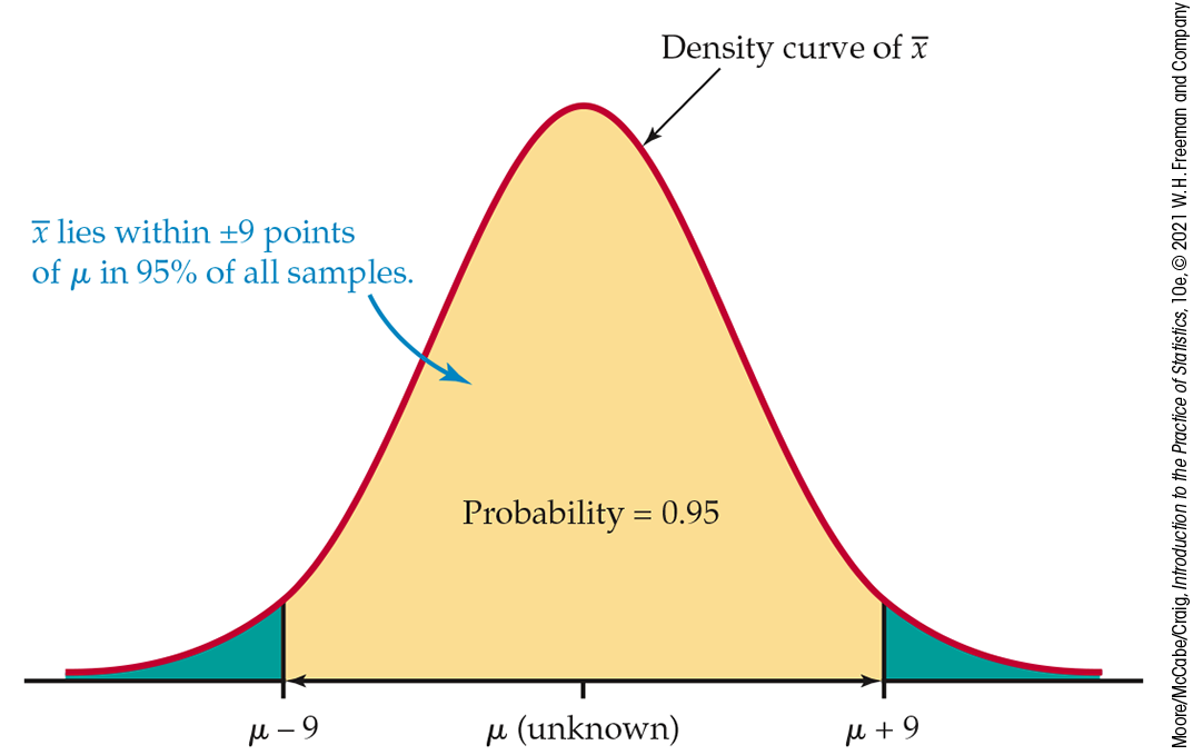
Figure 6.2 Distribution of the sample mean, Example 6.3.
We have simply restated a fact about the sampling distribution of
and
Be sure you understand the grounds for our confidence. There are only two possibilities for our SRS:
-
The interval between 496 and 514 contains the true
-
The interval between 496 and 514 does not contain the true
We cannot know whether our sample is one of the 95% for which the
interval
Check-in
-
6.1 How much do you spend on lunch? The average amount you spend on a lunch during the week is not known. Based on past experience, you are willing to assume that the standard deviation is $1.75. If you take a random sample of 25 lunches, what is the value of the standard deviation of
-
6.2 Applying the 68–95–99.7 rule. In the setting of the previous Check-in question, the 68–95–99.7 rule says that the probability is about 0.95 that
-
6.3 Constructing a 95% confidence interval. In the setting of the previous two Check-in questions, about 95% of all samples will capture the true mean in the interval
Confidence intervals
In the setting of
Example 6.3,
the interval of numbers between the values
The estimate
Figure 6.3
illustrates the behavior of 95% confidence intervals in repeated
sampling from a Normal distribution with mean
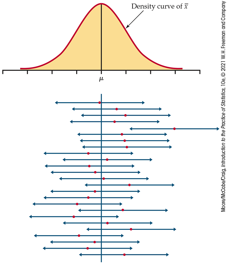
Figure 6.3 Twenty-five
samples from the same population gave these 95% confidence
intervals. In the long run, 95% of all samples give an interval
that covers
The 95% confidence intervals,
We can construct confidence intervals for many different parameters based on a variety of designs for data collection. We will learn the details of a number of these in later chapters. Two important things about a confidence interval are common to all settings:
- It is an interval of the form (a, b), where a and b are numbers computed from the sample data.
- It has a property called a confidence level that gives the probability of producing an interval that contains the unknown parameter.
Users can choose the confidence level, but 95% is the standard for
most situations. Occasionally, 90% or 99% is used. We use C to
stand for the confidence level in decimal form. For example, a 95%
confidence level corresponds to
![]() With the Confidence Intervals applet, you can construct
diagrams similar to the one displayed in
Figure 6.3. The
only differences are that the applet displays both the Normal
population distribution and the Normal sampling distribution of
With the Confidence Intervals applet, you can construct
diagrams similar to the one displayed in
Figure 6.3. The
only differences are that the applet displays both the Normal
population distribution and the Normal sampling distribution of
The spread of the data for the latest SRS reflects the spread of the
population distribution. This spread is assumed known, and it does not
change with sample size. What does change, as you vary n, is
the spread of the sampling distribution of
Check-in
-
 6.4 Generating a single confidence interval.
Set the Confidence Intervals applet to a 95% confidence
level and
6.4 Generating a single confidence interval.
Set the Confidence Intervals applet to a 95% confidence
level and
-
Is the spread in the data, shown as dots below the confidence interval, larger than the span of the confidence interval? Explain why this would typically be the case.
-
For the same data set, you can compare the span of the confidence interval for different values of C by sliding the confidence level to a new value. For the SRS you generated in part (a), what happens to the span of the interval when you move C to 99%? What about 90%? Describe the relationship you find between the confidence level C and the span of the confidence interval.
-
-
6.5 80% confidence intervals.
The idea of an 80% confidence interval is that the interval
captures the true parameter value in 80% of all samples. That’s
not high enough confidence for practical use, but 80% hits and
20% misses make it easy to see how a confidence interval behaves
in repeated samples from the same population.
-
Set the confidence level in the Confidence Intervals applet to 80% and
-
We can’t determine whether a new SRS will result in an interval that contains
-
Confidence interval for a population mean
![]()
We now construct a level C confidence interval for the mean
Our construction of a 95% confidence interval for the mean SATM score
began by noting that any Normal distribution has probability about
0.95 within
Because all Normal distributions have the same standardized form, we
can obtain everything we need from the standard Normal curve.
Figure 6.4
shows how C and
|
|
1.645 | 1.960 | 2.576 |
| C | 90% | 95% | 99% |
Notice that for 95% confidence, the value 2 obtained from the 68–95–99.7 rule is replaced with the more precise 1.96.
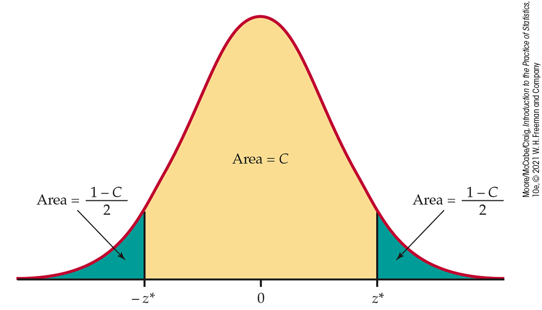
Figure 6.4 To construct
a level C confidence interval, we must find the number
As
Figure 6.4
reminds us, any Normal curve has probability C between the
point
This is exactly the same as saying that the unknown population mean
That is, there is probability C that the interval
Since 2008, Sallie Mae, a major provider of education loans and savings programs, has conducted an annual study titled “How America Pays for College.” In the 2019 survey, 2000 randomly selected individuals (1000 parents of undergraduate students and 1000 undergraduate students) were surveyed online.4
Many of the survey questions focus on the composition of funding sources used to pay for college, so the undergraduates in the survey are often responding for their family. For example, each participant is asked to report how much of the parents’ current income is used to pay for college. Do you think it is wise to combine responses across the parents and undergraduates? Are you fully aware of how much money your parents are spending and borrowing for college? The authors consider this one population and report overall averages and percents in their report. We will also consider this a sample from one population, but this is certainly debatable.
Example 6.4 Average college savings fund contribution.
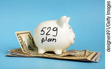
One Sallie Mae survey question asked how much money from a college savings fund, such as a 529 plan, is used to pay for college. Of the 2000 who were surveyed, the average amount is $1577. This population distribution is highly skewed to the right, with many zeros and likely a few very large amounts. Nevertheless, because the sample size is quite large, we can rely on the central limit theorem to assure us that the confidence interval based on the Normal distribution will be a good approximation.
Let’s compute an approximate 95% confidence interval for the true
mean amount contributed from a college savings fund among all
undergraduates. We’ll assume that the standard deviation for the
population of college savings fund contributions is $2076. For 95%
confidence, we see from
Table D
that
We have computed the margin of error with more digits than we really
need. Our mean is rounded to the nearest $1, so we will do the same
for the margin of error. Keeping additional digits would provide no
additional useful information. Therefore, we will use
We are 95% confident that the mean amount contributed from a college savings fund among all undergraduates is between $1486 and $1668.
Suppose that the researchers who designed this study had used a different sample size. How would this affect the confidence interval? We can answer this question by changing the sample size in our calculations and assuming that the sample mean is the same.
Example 6.5 How sample size affects the confidence interval.
As in Example 6.4, the sample mean of the college savings fund contribution is $1577, and the population standard deviation is $2076. Suppose that the sample size is only 500, but it is still large enough for us to rely on the central limit theorem. In this case, the margin of error for 95% confidence is
and the approximate 95% confidence interval is
Notice that the margin of error for this example is twice as large as the margin of error that we computed in Example 6.4. The only change that we made was to assume that the sample size is 500 rather than 2000. This sample size is one-fourth of the original 2000. Thus, we double the margin of error when we reduce the sample size to one-fourth of the original value. Figure 6.5 illustrates the effect in terms of the intervals.
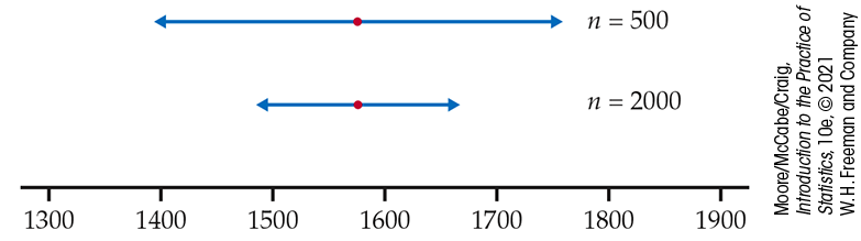
Figure 6.5 Confidence
intervals for
Check-in
-
6.6 Average amount paid for college. Refer to Example 6.4. The average annual amount the
The argument leading to the form of confidence intervals for the
population mean
The estimate based on the sample is the center of the confidence
interval. The margin of error is
How confidence intervals behave
The margin of error
Both high confidence and a small margin of error are desirable characteristics of a confidence interval. High confidence says that our method almost always gives correct answers. A small margin of error says that we have pinned down the parameter quite precisely.
Suppose that in planning a study, you calculate the margin of error and decide that it is too large. Here are your choices to reduce it:
- Use a lower level of confidence (smaller C).
- Choose a larger sample size (larger n).
-
Reduce
For most problems, you would choose a confidence level of 90%, 95%, or
99%, so
Example 6.6 How the confidence level affects the confidence interval.
Suppose that for the college saving fund contribution data in
Example 6.4
(page 336), we
wanted 99% confidence.
Table D
tells us that for 99% confidence,
and the 99% confidence interval is
Requiring 99%, rather than 95%, confidence has increased the margin of error from 91 to 120. Figure 6.6 compares the two intervals.
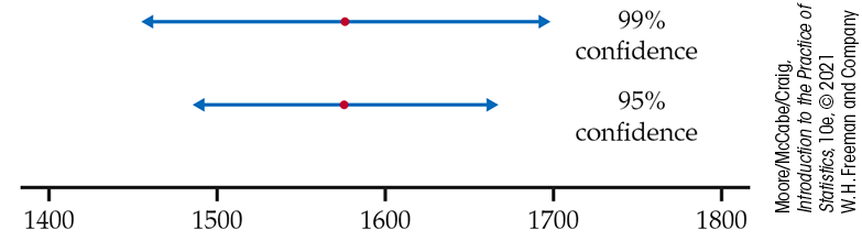
Figure 6.6 Confidence intervals, Examples 6.4 and 6.6. The larger the value of C, the wider the interval.
Similarly, choosing a larger sample size n reduces the margin
of error for any fixed confidence level. The square root in the
formula implies that we must multiply the number of observations by 4
in order to cut the margin of error in half. Likewise, if we want to
reduce the standard deviation of
The standard deviation
Check-in
-
6.7 Changing the sample size. In the setting of Check-in question 6.6 (page 338), would the margin of error for 95% confidence be doubled or halved if the sample size were raised to
-
6.8 Changing the confidence level. In the setting of Check-in question 6.6 (page 338), would the margin of error for 90% confidence be larger or smaller? Verify your answer by performing the calculations.
Choosing the sample size
A wise user of statistics never plans data collection without, at the same time, planning the inference. You can arrange to have both high confidence and a small margin of error through the margin of error formula for a population mean
By rearranging this equation, we can find the sample size n for a desired margin of error m. Here is the result.
Recall that the value of
A drawback of this formula is that it does not account for collection costs. In practice, taking observations costs time and money. The required sample size may be impossibly expensive. If you face such a situation, you might consider a larger margin of error and/or a lower confidence level to find a workable sample size.
![]() This formula also does not adjust for the fact that the actual
number of usable observations is often less than what is planned at
the beginning of a study.
This is particularly true of data collected in surveys but is an
important consideration in most studies. Careful study designers often
assume a nonresponse rate or dropout rate that specifies what
proportion of the originally planned sample will fail to provide data.
This information is used to adjust the sample size to be used at the
start of the study.
This formula also does not adjust for the fact that the actual
number of usable observations is often less than what is planned at
the beginning of a study.
This is particularly true of data collected in surveys but is an
important consideration in most studies. Careful study designers often
assume a nonresponse rate or dropout rate that specifies what
proportion of the originally planned sample will fail to provide data.
This information is used to adjust the sample size to be used at the
start of the study.
Example 6.7 How many undergraduates should we survey?
Suppose that we are planning a survey similar to the one described in Example 6.4 (page 336). If we want the margin of error for the average amount contributed from a college savings plan to be $50 with 95% confidence, what sample size n do we need?
For 95% confidence,
Table D
gives
Because
If past studies suggested that 70% of those contacted will respond, we
would need to start with a sample size of
The purpose of these calculations is to determine a sample size that
is sufficient to provide useful results, but the determination of what
is useful is a matter of judgment that requires subject-matter
knowledge. In
Section 7.3
(page 433), we
revisit this issue of sample size determination under the more
realistic setting when
Check-in
-
6.9 Starting salaries. You are planning a survey of starting salaries for recent computer science majors. In the latest survey by the National Association of Colleges and Employers, the average starting salary was reported to be $68,668.6 If you assume that the standard deviation is $6650, what sample size do you need in order to have a margin of error equal to $500 with 95% confidence?
-
6.10 Changes in sample size. Suppose that in the setting of the previous Check-in question you have the resources to contact 1000 recent graduates. If all respond, will your margin of error be larger or smaller than $500? What if only 60% respond? Verify your answers by computing the margin of errors.
Some cautions
We have already seen that small margins of error and high confidence
can require large numbers of observations.
![]() You should also be keenly aware that any formula for inference is
correct only in specific circumstances. If the government required statistical procedures to carry warning
labels like those on drugs, most inference methods would have long
labels. Our formula
You should also be keenly aware that any formula for inference is
correct only in specific circumstances. If the government required statistical procedures to carry warning
labels like those on drugs, most inference methods would have long
labels. Our formula
- The data should be an SRS from the population. However, we are not in great danger if the data can plausibly be thought of as independent observations from a population. That is the case in Examples 6.4 through 6.7, provided that the undergraduates and parents can be considered one population.
- The formula is not correct for probability sampling designs more complex than an SRS. Correct methods for other designs are available. If you plan such samples, be sure that you (or your statistical consultant) know how to carry out the inference you desire.
- There is no correct method for inference from data haphazardly collected with bias of unknown size. Fancy formulas cannot rescue badly produced data.
-
Because
-
If the sample size is small and the population is not Normal, the
true confidence level will be different from the value C used
in computing the interval.
Prior to doing any calculations, examine your data carefully for
skewness and other signs of non-Normality.
Remember, though, that the
interval relies only on the distribution of
-
The interval
The most important caution concerning confidence intervals is a consequence of the first of these warnings. The margin of error in a confidence interval covers only random sampling errors. The margin of error is obtained from the sampling distribution and indicates how much error can be expected because of chance variation in randomized data production.
![]() Practical difficulties such as undercoverage and nonresponse in a
sample survey cause additional errors. These errors can be larger
than the random sampling error.
This often happens when the sample size is large (so that
Practical difficulties such as undercoverage and nonresponse in a
sample survey cause additional errors. These errors can be larger
than the random sampling error.
This often happens when the sample size is large (so that
Every inference procedure that we will meet has its own list of warnings. Because many of the warnings are similar to those we have mentioned, we will not print the full warning label each time. It is easy to state (from the mathematics of probability) conditions under which a method of inference is exactly correct. These conditions are never fully met in practice.
For example, no population is exactly Normal. Deciding when a statistical procedure should be used in practice often requires judgment assisted by exploratory analysis of the data. Mathematical facts are, therefore, only a part of statistics. The difference between statistics and mathematics can be stated thusly: mathematical theorems are true; statistical methods are often effective when used with skill.
Finally, you should understand what statistical confidence does not say. Based on our SRS in Example 6.3, we are 95% confident that the mean SATM score for the California students lies between 496 and 514. This says that this interval was calculated by a method that gives correct results in 95% of all possible samples. It does not say that the probability is 0.95 that the true mean falls between 496 and 514. No randomness remains after we draw a particular sample and compute the interval. The true mean either is or is not between 496 and 514. The probability calculations of standard statistical inference describe how often the method, not a particular sample, gives correct answers.
Check-in
-
6.11 Nonresponse in a survey. In earlier versions of the Sallie Mae survey of Example 6.4 (page 336), participants were asked to report the undergraduate’s outstanding credit card balance. Only about a third reported this amount. Provide a couple of reasons why a survey respondent might not provide an amount. Based on these reasons, do you think the sample mean using just the reported amounts is biased? Is the margin of error based just on the reported amounts a good measure of precision? Explain your answers.
Section 6.1 SUMMARY
-
The purpose of a confidence interval is to estimate an unknown parameter with an indication of how accurate the estimate is and of how confident we are that the result is correct.
-
Any confidence interval has two parts: an interval computed from the data and a confidence level. The interval often has the form
-
The confidence level states the probability that the method will give a correct answer. That is, if you use 95% confidence intervals, in the long run 95% of your intervals will contain the true parameter value. When you apply the method once (that is, to a single sample), you do not know if your interval gave a correct answer (which happens 95% of the time) or not (which happens 5% of the time).
-
Other things being equal, the margin of error of a confidence interval decreases as
- – The confidence level C decreases.
- – The sample size n increases.
-
– The population standard deviation
-
The level C margin of error of
Here
-
The level C confidence interval for
If the population is not Normal and n is large, the confidence level of this interval is approximately correct.
-
The sample size n required to obtain a confidence interval of specified margin of error m for a population mean is
where
-
A specific confidence interval formula is correct only under specific conditions. The most important conditions concern the method used to produce the data. Other factors such as the form of the population distribution may also be important. These conditions should be investigated prior to doing any calculations.
Section 6.1 EXERCISES
-
6.1 Student loan debt. The average student loan debt among college graduates is reported using the 95% confidence interval ($23,923, $34,447).
-
Describe what this interval tells us about average student loan debt.
-
What is the estimated average student loan debt among college graduates?
What is the margin of error?
-
-
6.2 Margin of error and the confidence interval. A study of stress on the campus of your university using the College Undergraduate Stress Scale (CUSS) reported an average stress level of 1123 (a higher score indicating more stress) with a margin of error of 43 for 95% confidence. The study was based on a random sample of 400 undergraduates.
Give the 95% confidence interval.
-
If you wanted 99% confidence for the same study, would your margin of error be greater than, equal to, or less than 43? Explain your answer.
-
6.3 Changing the sample size. Consider the setting of the previous exercise. Suppose that the sample mean is again 1123, and the population standard deviation is 441. Make a diagram similar to Figure 6.5 (page 338) that illustrates the effect of sample size on the width of a 95% interval. Use the following sample sizes: 100, 144, 225, 324, and 400. Summarize what the diagram shows.
-
6.4 Changing the confidence level. Consider the setting of the previous two exercises. Suppose that the sample mean is still 1123, the sample size is 400, and the population standard deviation is 441. Make a diagram similar to Figure 6.6 (page 339) that illustrates the effect of the confidence level on the width of the interval. Use 80%, 90%, 95%, and 99%. Summarize what the diagram shows.
-
6.5 Confidence interval mistakes and misunderstandings. Suppose that 500 randomly selected alumni of the University of Okoboji were asked to rate the university’s academic advising services on a scale of 1–10. The sample mean
-
Ima Bitlost computes the 95% confidence interval for the average satisfaction score as
-
After correcting her mistake in part (a), Ima states, “I am 95% confident that the sample mean falls between 8.4 and 8.8.” What is wrong with this statement?
-
Ima quickly realizes her mistake in part (b) and instead states, “The probability that the true mean is between 8.4 and 8.8 is 0.95.” What misinterpretation is she making now?
-
Finally, in her defense for using the Normal distribution to determine the confidence interval, Ima says, “Because the sample size is quite large, the population of alumni ratings will be approximately Normal.” Explain to Ima her misunderstanding and correct this statement.
-
-
6.6 More confidence interval mistakes and misunderstandings. Suppose that 100 randomly selected subscribers of Stingray Karaoke on YouTube asked how much time they typically spend on the site during the week.7 The sample mean
-
Cary Oakey computes the 95% confidence interval for the average time on the site as
-
Cary corrects this mistake and then states that “95% of the members spend between 2.03 and 2.77 hours a week on the site.” What is wrong with his interpretation of this interval?
-
To reduce the margin of error in half, Cary says that the sample size needs to be doubled to 200. What is wrong with this statement?
-
-
6.7 The state of stress in the United States. Since 2007, the American Psychological Association has supported an annual nationwide survey to examine stress across the United States.8 This year, a total of 3602 adults were asked to indicate their average stress level (on a 10-point scale) during the past month.
-
For the 343 Gen Z adults (18- to 22-year-olds), the mean score was 5.5. Assuming that the population standard deviation is 2.9, give the margin of error and find the 95% confidence interval for the mean Gen Z stress level.
-
In addition, all survey respondents were asked to state what they regarded to be a “healthy” stress level. The mean score was 3.8. Assuming a population standard deviation of 2.2, give the margin of error and find the 95% confidence interval for the mean.
-
Compare the two intervals. Do you think we can conclude that Gen Z adults have an average stress level that is above what is considered healthy? Explain your answer.
-
-
6.8 Inference based on integer values. Refer to Exercise 6.7. The data for this study are integer values between 1 and 10. Explain why the confidence interval for the mean
-
6.9 Mean TRAP in young women. For many important processes that occur in the body, direct measurement of characteristics of the process is not possible. In many cases, however, we can measure a biomarker, a biochemical substance that is relatively easy to measure and is associated with the process of interest. Bone turnover is the net effect of two processes: the breaking down of old bone, called resorption, and the building of new bone, called formation. One biochemical measure of bone resorption is tartrate-resistant acid phosphatase (TRAP), which can be measured in blood. In a study of bone turnover in young women, serum TRAP was measured in 31 subjects.9 The mean was 13.2 units per liter (U/l). Assume that the standard deviation is known to be 6.5 U/l. Give the margin of error and find a 95% confidence interval for the mean TRAP amount in young women represented by this sample.
-
6.10 Mean OC in young women. Refer to the previous exercise. A biomarker for bone formation measured in the same study was osteocalcin (OC), measured in the blood. For the 31 subjects in the study, the mean was 33.4 nanograms per milliliter (ng/ml). Assume that the standard deviation is known to be 19.6 ng/ml. Report the 95% confidence interval.
-
6.11 Populations sampled and margins of error. Consider the following two scenarios. (A) Take a simple random sample (SRS) of 250 first-year students at your college or university. (B) Take an SRS of 250 students at your college or university. For each of these samples, you will record the amount spent on textbooks used for classes during the fall semester. Which sample should have the smaller margin of error? Explain your answer.
-
 6.12 Average starting salary. The National
Association of Colleges and Employers (NACE) Summer Salary
Survey shows that the current class of college graduates
received an average starting-salary offer of $50,994.10
Your institution collected an SRS
6.12 Average starting salary. The National
Association of Colleges and Employers (NACE) Summer Salary
Survey shows that the current class of college graduates
received an average starting-salary offer of $50,994.10
Your institution collected an SRS -
6.13 Consumption of sweet snacks. A study reported that the U.S. per capita consumption of sweet snacks among healthy-weight children aged 12 to 19 years is 251.2 kilocalories per day (kcal/d).11 This was based on 24-hour dietary recall records of
-
Suppose that the population distribution is heavily skewed, with a standard deviation equal to 540 kcal/d. What is the margin of error for a 95% confidence interval of the per capita consumption of sweet snacks?
-
A future study is being planned, and the goal is to have the margin of error no more than 15 kcal/d. Based on your answer to part (a), will this study require an examination of more or fewer 24-hour dietary recall records? Explain your answer without calculations.
-
Based on your answer in part (b), will more or fewer recall records be required if the confidence level is increased to 99%? Again explain your answer without calculations.
-
Compute the sample sizes necessary for the studies described in parts (b) and (c).
-
-
6.14 Total sleep time of college students. In Example 5.4 (page 282), the total sleep time per night among college students was approximately Normally distributed with mean
-
What is the standard deviation of the sample mean in hours? In minutes?
-
Use the 95 part of the 68–95–99.7 rule to describe the variability of this sample mean.
-
What is the probability that your sample average will be below 7.0 hours?
-
-
6.15 Determining sample size. Refer to the previous exercise. You really want to use a sample size such that about 95% of the averages fall within
-
Based on your answer to part (b) in Exercise 6.14, should the sample size be larger or smaller than 175? Explain your answer.
-
What standard deviation of
-
Using the standard deviation you calculated in part (b), determine the number of students you need to sample in order to achieve this.
-
-
6.16 Inference based on skewed data. The mean
OC for the 31 subjects in
Exercise 6.10
was 33.4 ng/ml. In our calculations, we assumed that the
standard deviation was known to be 19.6 ng/ml. Use the
68–95–99.7 rule from
Chapter 1 (page 51) to find the approximate bounds on the values of OC that would
include these percents of the population. If the assumed
standard deviation is correct, this distribution may be highly
skewed. Why? (Hint: The measured values for a variable
such as this are all positive.) Do you think that this skewness
will invalidate the use of the Normal confidence interval in
this case? Explain your answer.
-
6.17 Average hours per week listening to audio. An iHeartMedia-sponsored survey of 6016 consumers who listen at least once a week to an audio platform reported an average of 17.2 hours a week listening to audio, such as broadcast radio, streaming music services, and podcasts.12 Assume that the standard deviation is 6.8 hours.
-
Give a 95% confidence interval for the mean time spent per week listening to audio.
-
Is it true that 95% of the 6016 consumers reported weekly times that lie in the interval you found in part (a)? Explain your answer.
-
It is likely this population distribution is very skewed with many small listening times and several very large times. Explain why the confidence interval based on the Normal distribution should nevertheless be a good approximation in this case.
-
-
6.18 Average minutes per week listening to audio. Refer to the previous exercise.
-
Give the sample mean and sample standard deviation in minutes.
-
Calculate the 95% confidence interval in minutes from your answers to part (a).
-
Explain how you could have directly calculated this interval from the 95% interval that you calculated in the previous exercise.
-
-
6.19 Outlook on life. Since 2008, the Gallup-Sharecare Well-Being Index tracks how people feel about their daily lives. In 2017, 56.3% of the respondents were classified as “thriving.” This classification is based on how a respondent rates his or her current and future lives. This is the highest percent of respondents in this category since the index started. Material provided with the results noted:
Results are based on telephone interviews. . . with a random sample of 160,498 adults, living in all 50 U.S. states and the District of Columbia. For results based on the total sample of national adults, the margin of sampling error is
The poll uses a complex multistage sample design, but the sample percent has approximately a Normal sampling distribution.
-
The announced poll result was
-
Explain to someone who knows no statistics what the announced result
-
This confidence interval has the same form we have met earlier:
What is the standard deviation
-
Does the announced margin of error include errors due to practical problems such as nonresponse? Explain your answer.
-
-
6.20 How many “hits”? The
Confidence Intervals applet lets you simulate large
numbers of confidence intervals quickly. Select 95% confidence
and then sample 50 intervals. Record the number of intervals
that cover the true value. Repeat this process until you have 30
counts of hits. Make a stemplot or histogram of the results and
find the mean. Describe the results. If you repeated this
experiment very many times, what would you expect the average
number of hits to be?
-
6.21 Required sample size for specified margin of error. A new bone study is being planned that will measure the biomarker TRAP described in Exercise 6.9. Using the value of
-
6.22 Adjusting required sample size for dropouts.
Refer to the previous exercise. In similar previous studies,
about 20% of the subjects drop out before the study is
completed. Adjust your sample size requirement so that you will
have enough subjects at the end of the study to meet the margin
of error criterion.
-
6.23 Radio poll. A National Public Radio (NPR) station invites listeners to enter a dispute about a proposed “pay as you throw” waste collection program. The station asks listeners to call in and state how much each 10-gallon bag of trash should cost. A total of 179 listeners call in. The station calculates the 95% confidence interval for the average fee to be $0.53 to $1.39. Is this result trustworthy? Explain your answer.
-
6.24 Accuracy of a laboratory scale. To assess the accuracy of a laboratory scale, a standard weight known to weigh 10 grams is weighed repeatedly. The scale readings are Normally distributed with unknown mean. (This mean is 10 grams if the scale has no bias.) The standard deviation of the scale readings is known to be 0.0002 gram.
-
The weight is measured six times. The mean result is 10.0023 grams. Give a 99% confidence interval for the mean of repeated measurements of the weight.
-
Based on the interval in part (a), do you think the scale is accurate? Explain your answer.
-
How many measurements must be averaged to get a margin of error of
-
-
6.25 More than one confidence interval.
As we prepare to take a sample and compute a 95% confidence
interval, we know that the probability that the interval we
compute will cover the parameter is 0.95. That’s the meaning of
95% confidence. If we plan to use several such intervals,
however, our confidence that all of them will give
correct results is less than 95%. Suppose that we plan to take
independent samples each month for five months and report a 95%
confidence interval for each set of data.
-
What is the probability that all five intervals will cover the true means? This probability (expressed as a percent) is our overall confidence level for the five simultaneous statements.
-
Suppose we instead considered individual 99% confidence intervals. Now, what is the overall confidence level for the five simultaneous statements?
-
Based on the results of parts (a) and (b), how could you keep the overall confidence level near 95% if you were considering 10 simultaneous intervals?
-