8.2 Comparing Two Proportions
In studies about proportions, it is far more common to compare the proportions of two groups (such as subjects in a treatment group versus those in a control group). In the previous section, we learned the methods of inference for a single proportion. Our problem now concerns the comparison of two proportions.
Similar to our approach when comparing two means (page 410), we call the two groups being compared Population 1 and Population 2
and the two population proportions of “successes”
| Population | Population proportion | Sample size | Count of successes | Sample proportion |
|---|---|---|---|---|
| 1 |
|
|
|
|
| 2 |
|
|
|
|
To compare the two populations, we use the difference between the two sample proportions:
When both sample sizes are sufficiently large, the sampling distribution of the difference D is approximately Normal.
EXAMPLE 8.11 Lost wallets.
![]()

If you lose your wallet, what is the chance that it will be returned to you? Does this chance depend on whether or not there is money in your wallet? The answer is somewhat surprising. A recent study collected data from 355 cities in 40 countries. Researchers designed experiments to examine these questions. For the United States, there were 300 wallets with no money and 300 wallets with money ($13.45).16 Here are the results:
| Wallet condition | n | X |
|
|---|---|---|---|
| Money | 300 | 174 | 0.58 |
| No money | 300 | 111 | 0.37 |
In each row of this table, X is the number of wallets returned,
and
Inference procedures for comparing proportions are z procedures based on the Normal approximation and on standardizing the difference D. The first step is to obtain the mean and standard deviation of D. By the addition rule for means, the mean of D is the difference of the means:
That is, the difference
Therefore, when
Check-in
-
8.14 Rules for means and variances. Suppose that
-
8.15 Effect of the sample sizes. Suppose that
-
Find the mean and the standard deviation of the sampling distribution of
-
The sample sizes here are four times as large as those in the previous Check-in question, but the population proportions are the same. Compare the results for this Check-in question with those that you found in the previous Check-in question. What is the effect of multiplying the sample sizes by 4?
-
-
8.16 Verify the formulas. It is quite easy to verify the formulas for the mean and standard deviation of the difference D.
-
What are the means and standard deviations of the two sample proportions
-
Use the addition rule for means of random variables. What is the mean of
-
The two samples are independent. Use the addition rule for variances of random variables. What is the variance of D?
-
Large-sample confidence interval for a difference in proportions
To obtain a confidence interval for
Example 8.12 Confidence interval for lost wallets.
Let’s find a 95% confidence interval for the difference between the proportions of returned wallets with money and with no money. From Example 8.11 we know
| Wallet condition | n | X |
|
|---|---|---|---|
| Money | 300 | 174 | 0.58 |
| No money | 300 | 111 | 0.37 |
and
To get the margin of error, we first calculate the standard error of D:
For 95% confidence, we have
The 95% confidence interval is
With 95% confidence, we can say that the difference in the proportions is between 0.1319 and 0.2881. Alternatively, we can report that the difference between the percent returned of wallets with money and the percent returned of wallets with no money is 21.0%, with a 95% margin of error of 7.8%.
In this example, we chose wallets with money as the first population.
Had we chosen wallets with no money to be the first population, the
estimate of the difference would be negative
Example 8.13 Lost wallets confidence interval from software.
![]()
Figure 8.5 shows a spreadsheet that can be used as input to software. Separate columns label each count according to condition and response. Output from JMP and Minitab is given in Figure 8.6. Compare these outputs with the calculations that we performed in Example 8.11.
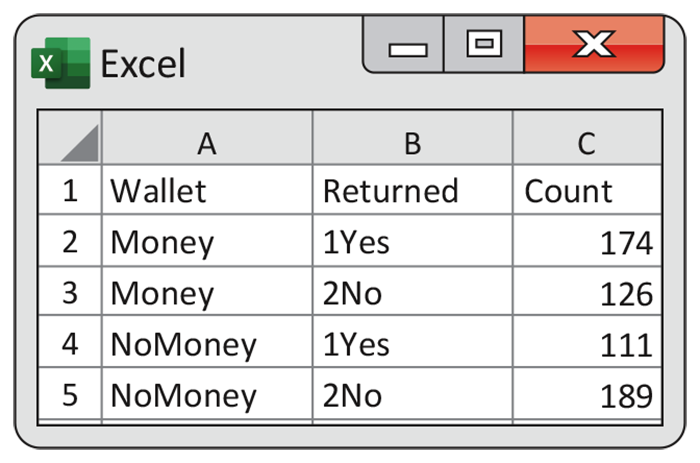
Figure 8.5 Spreadsheet that can be used as input to software that computes the confidence interval for the lost wallet data, Example 8.13.
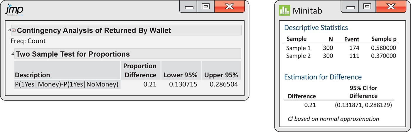
Figure 8.6 JMP and Minitab outputs for the lost wallet confidence interval, Example 8.13.
![]()
Check-in
-
8.17 Age and commercial preference. A study was designed to compare two energy drink commercials. Participants were individuals aged 18 to 25 who regularly drink energy drinks. Each participant was shown the commercials in random order and asked to select the better one. Commercial A was selected by 46 out of the 103 participants aged 18 to 21 years and by 65 out of the 110 participants aged 22 to 25 years. Give an estimate of the difference in age proportions that favored Commercial A. Also construct a large-sample 95% confidence interval for this difference.
-
8.18 Confidence interval for age and commercial preference. Refer to the previous Check-in question. Construct a 95% confidence interval for the difference in proportions that favor Commercial B. Explain how you could have obtained these results from the calculations you did in Check-in question 8.17.
Example 8.14 Plus four for sex and sexual maturity.
In studies that look for a difference between sexes, a major concern is whether or not apparent differences are due to other variables that are associated with sex. Because boys mature more slowly than girls, a study of adolescents that compares boys and girls of the same age may confuse a sex effect with an effect of sexual maturity. The “Tanner score” is a commonly used measure of sexual maturity.18 Subjects are asked to determine their score by placing a mark next to a rough drawing of an individual at their level of sexual maturity. There are five different drawings, so the score is an integer between 1 and 5.
A pilot study included 12 girls and 12 boys from a population that will be used for a large experiment. Four of the boys and three of the girls had Tanner scores of 4 or 5, a high level of sexual maturity. Let’s find a 95% confidence interval for the difference between the proportions of boys and girls who have high (4 or 5) Tanner scores in this population. The numbers of successes and failures in both groups are not all at least 10, so the large-sample approach is not recommended. On the other hand, the sample sizes are both at least 5, so the plus four method is appropriate.
The plus four estimate of the population proportion for boys is
For girls, the estimate is
Therefore, the estimate of the difference is
The standard error of
For 95% confidence,
The confidence interval is
With 95% confidence we can say that the difference in the
proportions is between
The very large margin of error in this example indicates that either
boys or girls could be more sexually mature in this population and
that the difference could be quite large.
Although the interval includes the possibility that there is no
difference, corresponding to
![]() With small sample sizes such as these, the data do not provide us
with a lot of information for our inference. This fact is expressed
quantitatively through the very large margin of error.
With small sample sizes such as these, the data do not provide us
with a lot of information for our inference. This fact is expressed
quantitatively through the very large margin of error.
Significance test for a difference in proportions
![]()
Although we prefer to compare two proportions by giving a confidence interval for the difference between the two population proportions, it is sometimes useful to test the null hypothesis that the two population proportions are the same.
We standardize
If
We estimate the common value of p by the overall proportion of successes in the two samples:
This is called the
pooled
estimate of
To estimate
The subscript on
Example 8.15 Lost wallets: The z test.
![]()
Are wallets with no money and wallets with money equally likely to be returned? We examine the data in Example 8.11 (page 469) to answer this question. Here is the data summary:
| Wallet condition | n | X |
|
|---|---|---|---|
| Money | 300 | 174 | 0.58 |
| No money | 300 | 111 | 0.37 |
The sample proportions are certainly quite different, but we will perform a significance test to see if the difference is large enough to lead us to believe that the population proportions are not equal. Formally, we test the hypotheses
The pooled estimate of the common value of p is
The test statistic is calculated as follows:
The P-value is
Here is our summary: 58% of the wallets with money and 37% of the
wallets with no money were returned; the difference is statistically
significant
Example 8.16 Output for the lost wallets significance test.
![]()
We prefer to use software to obtain the significance test results
for comparing the return rates of wallets with and without money.
Output from JMP and Minitab is given in
Figure 8.7. JMP reports the significance tests for the two-sided alternative
and for the two one-sided alternatives. We are interested in the
two-sided alternative. Therefore, we report the P-value as
<0.0001. Minitab reports the test statistic,
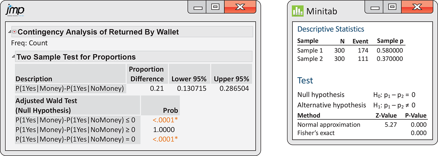
Figure 8.7 JMP and Minitab outputs for the lost wallet significance test, Example 8.16.
Do you think that we could have argued that the proportion would be
higher for wallets with money than for wallets without money before
looking at the data in this example? This would allow us to use the
one-sided alternative
Check-in
-
8.19 The z test for age and commercial preference. Refer to Check-in question 8.17 (page 472). Test whether the proportions of the two age groups are the same versus the two-sided alternative at the 5% level.
-
8.20 Changing the alternative hypothesis. Refer to Check-in question 8.19. Does your conclusion change if you perform the test with the older participants designated as the first group (corresponding to
Choosing a sample size for two sample proportions
In Section 8.1, we studied methods for determining the sample size using two settings. First, we used the margin of error for a single proportion as the criterion for choosing n (page 460). Second, we used the desired power of the significance test for a single proportion as the determining factor (page 462). We follow the same approach here for comparing two proportions.
Use the margin of error
Recall that the large-sample estimate of the difference in proportions is
the standard error of the difference is
and the margin of error for confidence level C is
where
For a single proportion, we guessed a value for the true proportion and computed the margins of error for various choices of n. Here we use the same idea, but we need to guess values for the two proportions. We can display the results in a table, as in Example 8.9 (page 461), or in a graph, as in Exercise 8.29 (page 467).
Example 8.17 Margin of error—based sample sizes for age and commercial preferences.
Consider the setting in
Check-in question 8.17, where we compared the preferences of two age groups for two
commercials. Suppose we want to do a study in which we perform a
similar comparison using a 95% confidence interval
that will have a margin of error of 0.2 or less. What should we
choose for our sample size? Using
We would include 48 participants in each age group for our study.
Note that we have rounded the calculated value, 48.02, down because
it is very close to 48 and we used
Check-in
-
8.21 What would the margin of error be? Consider the setting in Check-in question 8.17 with
-
Compute the margins of error for each of the following scenarios:
-
If you think that one of these scenarios is likely to fit your study, should you reconsider your choice of
-
Use the power of the significance test
When we studied using power to compute the sample size needed for a significance test for a single proportion, we used software. We will do the same for the significance test comparing two proportions.
Some software allows us to consider significance tests that are a
little more general than the version we studied in this section.
Specifically, we used the null hypothesis
Here is a summary of the inputs needed for software to perform the calculations:
- The significance level α (the probability of rejecting the null hypothesis when it is true); usually we choose 5% for the α.
- Power (probability of rejecting the null hypothesis when it is false); usually we choose 80% (0.80) for power.
-
The value of
-
The alternative hypothesis, two-sided
-
Values for
Example 8.18 Sample sizes for age and commercial preferences.
Refer to
Example 8.17, where
we used the margin of error to find the sample sizes for comparing
the preferences of two age groups for two commercials. Let’s find
the sample sizes required for a significance test that the two
proportions who prefer Commercial A are equal
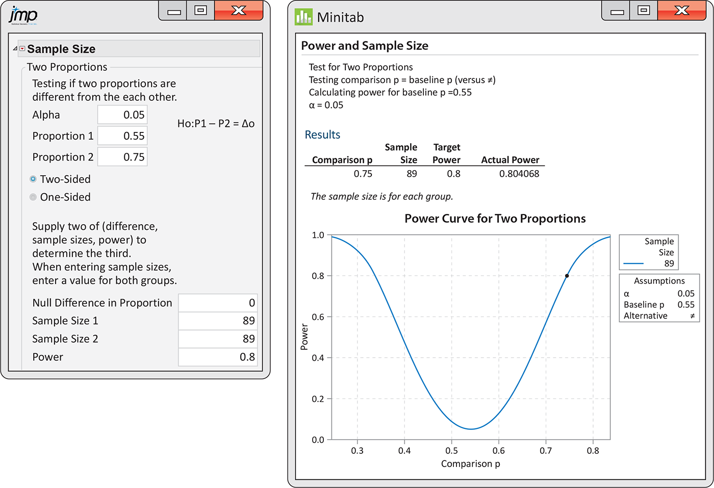
Figure 8.8 JMP and Minitab outputs for finding the sample size, Example 8.18.
Note that the Minitab output in
Figure 8.8
gives the power curve for different alternatives. All of these have
Check-in
-
8.22 Find the sample sizes. Consider the setting in Example 8.17. Change
Example 8.19 Aspirin and blood clots: Relative risk.

A study of 822 patients who completed a standard treatment for blood clots (venous thromboembolism) were randomly assigned in equal numbers to receive a low-dose aspirin or a placebo treatment. Patients were monitored for several years for the occurrence of several related medical conditions. Counts of patients who experienced one or more of these conditions were reported for each year after the study began.19 The following table gives the data for a composite of events, termed “major vascular events.” Here, X is the number of patients who had a major event during the time they were monitored:
| Population |
|
|
|
|---|---|---|---|
| 1 (aspirin) | 411 | 45 | 0.1095 |
| 2 (placebo) | 411 | 73 | 0.1776 |
| Total | 822 | 118 | 0.1436 |
The relative risk is
Software gives the 95% confidence interval as 0.4364 to 0.8707.
Taking aspirin has reduced the occurrence of major events to 62%
of what it is for patients taking the placebo. The 95% confidence
interval is 44% to 87%. The confidence interval does not include
1, so we conclude that the two proportions are different with
Note that the confidence interval is not symmetric about the estimate. Relative risk is one of many situations where this occurs.
Section 8.2 SUMMARY
-
The large-sample estimate of the difference in two population proportions is
where
-
The standard error of D is
-
The level C margin of error of D is
where
-
The level C large-sample confidence interval for D is
We recommend using this interval for 90%, 95%, or 99% confidence when the number of successes and the number of failures in both samples are all at least 10. When sample sizes are smaller, alternative procedures such as the plus four estimate of the difference in two population proportions are recommended.
-
Significance tests of
with P-values from the N(0, 1) distribution. In this statistic,
and
Use this test when the number of successes and the number of failures in each of the samples are at least 5.
-
Relative risk is the ratio of two sample proportions:
Confidence intervals for relative risk are often used to summarize the comparison of two proportions.
Section 8.2 EXERCISES
-
8.34 What’s wrong? For each of the following, explain what is wrong and why.
-
A z statistic is used to test the null hypothesis that
-
If two sample proportions are equal, then the sample counts are equal.
-
A 95% confidence interval for the difference in two proportions includes errors due to nonresponse.
-
-
8.35 Identify the key elements. For each of the following scenarios, identify the populations, the counts, and the sample sizes; compute the two proportions and find their difference.
-
A study of tipping behaviors examined the relationship between the color of the shirt worn by the server and whether or not the customer left a tip.20 There were 418 male customers in the study. Of the 69 customers served by a server wearing a red shirt, 40 left a tip. Of the 349 who were served by a server wearing a shirt of a different color, 130 left a tip.
-
A sample of 40 runners was used to compare two new routines for stretching. The runners were randomly assigned to one of the routines, which they followed for two weeks. Satisfaction with the routines was measured using a questionnaire at the end of the two-week period. For the first routine, 11 runners said that they were satisfied or very satisfied. For the second routine, 14 runners said that they were satisfied or very satisfied.
-
-
8.36 Apply the confidence interval guidelines. Refer to the previous exercise. For each of the scenarios, determine whether or not the guidelines for using the large-sample method for a 95% confidence interval are satisfied. Explain your answers.
-
8.37 Find the 95% confidence interval. Refer to Exercise 8.35. For each scenario, find the large-sample 95% confidence interval for the difference in proportions and use the scenario to explain the meaning of the confidence interval.
-
8.38 Apply the significance test guidelines. Refer to Exercise 8.35. For each of the scenarios, determine whether or not the guidelines for using the large-sample significance test are satisfied. Explain your answers.
-
8.39 Perform the significance test. Refer to Exercise 8.35. For each scenario, perform the large-sample significance test and use the scenario to explain the meaning of the significance test.
-
8.40 Teeth and military service. In 1898 the United States and Spain fought a war over the U.S. intervention in the Cuban War of Independence. At that time, the U.S. military was concerned about the nutrition of its recruits. Many did not have a sufficient number of teeth to chew the food provided to soldiers. As a result, it was likely that they would be undernourished and unable to fulfill their duties as soldiers. The requirements at that time specified that a recruit must have “at least four sound double teeth, one above and one below on each side of the mouth, and so opposed” so that they could chew food. Of the 58,952 recruits who were under the age of 20, 68 were rejected for this reason. For the 43,786 recruits who were 40 or over, 3801 were rejected.21
-
Find the proportion of rejects for each age group.
-
Find a 99% confidence interval for the difference in the proportions.
-
Use a significance test to compare the proportions. Write a short paragraph describing your results and conclusions.
-
Are the guidelines for the use of the large-sample approach satisfied for your work in parts (b) and (c)? Explain your answers.
-
-
8.41 Physical education requirements. In the 1920s, about 97% of U.S. colleges and universities required a physical education course for graduation. Today, about 40% require such a course. A recent study of physical education requirements included 354 institutions: 225 private and 129 public. Among the private institutions, 60 required a physical education course, while among the public institutions, 101 required a course.22
-
What are the explanatory and response variables for this exercise? Justify your answers.
What are the populations?
What are the statistics?
-
Use a 95% confidence interval to compare the private and the public institutions with regard to the physical education requirement.
-
Use a significance test to compare the private and the public institutions with regard to the physical education requirement.
-
For parts (d) and (e), verify that the guidelines for using the large-sample methods are satisfied.
-
Summarize your analysis of these data in a short paragraph.
-
-
8.42 Exergaming in Canada. Exergames are active video games such as rhythmic dancing games, virtual bicycles, balance board simulators, and virtual sports simulators that require a screen and a console. A study of exergaming practiced by students from grades 10 and 11 in Montreal, Canada, examined many factors related to participation in exergaming.23 Of the 358 students who reported that they stressed about their health, 29.9% said that they were exergamers. Of the 851 students who reported that they did not stress about their health, 20.8% said that they were exergamers.
-
Define the two populations to be compared for this exercise.
-
What are the counts, the sample sizes, and the proportions?
-
Are the guidelines for the use of the large-sample confidence interval satisfied?
-
Are the guidelines for the use of the large-sample significance test satisfied?
-
-
8.43 Confidence interval for exergaming in Canada. Refer to the previous exercise. Find the 95% confidence interval for the difference in proportions. Write a short statement interpreting this result.
-
8.44 Significance test for exergaming in Canada. Refer to Exercise 8.42. Use a significance test to compare the proportions. Write a short statement interpreting this result.
-
8.45 Adult gamers versus teen gamers. A Pew Internet Project Data Memo presented data comparing adult gamers with teen gamers with respect to the devices on which they play. The data are from two surveys. The adult survey had 1063 gamers, while the teen survey had 1064 gamers. The memo reports that 54% of adult gamers played on game consoles (Xbox, PlayStation, Wii, etc.), while 89% of teen gamers played on game consoles.24
-
Refer to the table that appears on page 468. Fill in the numerical values of all quantities that are known.
-
Find the estimate of the difference between the proportion of teen gamers who played on game consoles and the proportion of adults who played on these devices.
-
Is the large-sample confidence interval for the difference between two proportions appropriate to use in this setting? Explain your answer.
-
Find the 95% confidence interval for the difference.
-
Convert your estimated difference and confidence interval to percents.
-
The adult survey was conducted between October and December 2008, whereas the teen survey was conducted between November 2007 and February 2008. Do you think that this difference should have any effect on the interpretation of the results? Be sure to explain your answer.
-
-
8.46 Significance test for gaming on computers. Refer to the previous exercise. Test the null hypothesis that the two proportions are equal. Report the test statistic with the P-value and summarize your conclusion.
-
8.47 Gamers on computers. The report described in Exercise 8.45 also presented data from the same surveys for gaming on computers (desktops or laptops). These devices were used by 73% of adult gamers and by 76% of teen gamers. Answer the questions given in Exercise 8.45 for gaming on computers.
-
8.48 Significance test for gaming on consoles. Refer to the previous exercise. Test the null hypothesis that the two proportions are equal. Report the test statistic with the P-value and summarize your conclusion.
-
8.49 Find the sample size. You are planning a study in which you will use a 95% confidence interval to report the difference between two proportions. Find the sample size needed for a margin of error of 0.2 if you do not have good guess at the values of the two proportions. How would your answer change if you were willing to guess
-
8.50 Can we compare gaming on consoles with gaming on computers? Refer to Exercises 8.45 to 8.48. Do you think that you can use the large-sample confidence intervals for a difference in proportions to compare teens’ use of computers with teens’ use of consoles? Write a short paragraph giving the reason for your answer. (Hint: Look carefully at the assumptions needed for this procedure on page 470.)
-
8.51 Find the power. Consider testing the null hypothesis that two proportions are equal versus the two-sided alternative with
-
For each of the following situations, find the required sample size: (i)
Write a short summary describing your results.
-
-
8.52 Find the relative risk. Refer to Exercise 8.35. For each scenario, find the relative risk. Be sure to give a justification for your choice of proportions to use in the numerator and the denominator of the ratio. Use the scenarios to explain the meaning of the relative risk.