7.1 Inference for the Mean of a Population
Both confidence intervals and tests of significance for the mean
In this section, we meet the sampling distribution of the standardized
version of
The t distributions
Suppose that we have a simple random sample (SRS) of size
n from a Normally distributed population with mean
The term “standard error” is sometimes used for the actual standard deviation of a statistic. The estimated value is then called the “estimated standard error.” In this book, we will use the term “standard error” only when the standard deviation of a statistic is estimated from the data. The term has this meaning in the output of many statistical software packages and in research reports that apply statistical methods.
In the previous chapter, the standardized sample mean, or one-sample z statistic,
is the basis for inference about
A particular t distribution is specified by giving the degrees
of freedom. We use t(k) to stand for the
t distribution with k degrees of freedom. The degrees of
freedom for this t statistic come from the sample standard
deviation s in the denominator of t. We showed earlier
that s has
The t distributions were discovered in 1908 by William S. Gosset. Gosset was a statistician employed by the Guinness brewing company, which prohibited its employees from publishing their discoveries that were brewing related. In this case, the company let him publish under the pen name “Student” using an example that did not involve brewing. The t distribution is often called “Student’s t” in his honor.
The density curves of the t(k) distributions are similar in shape to the standard Normal curve. That is, they are symmetric about 0 and are bell-shaped. Figure 7.1 compares the density curves of the standard Normal distribution and the t distributions with 5 and 15 degrees of freedom. The similarity in shape is apparent, as is the fact that the t distributions have more probability in the tails and, thus, less in the center.
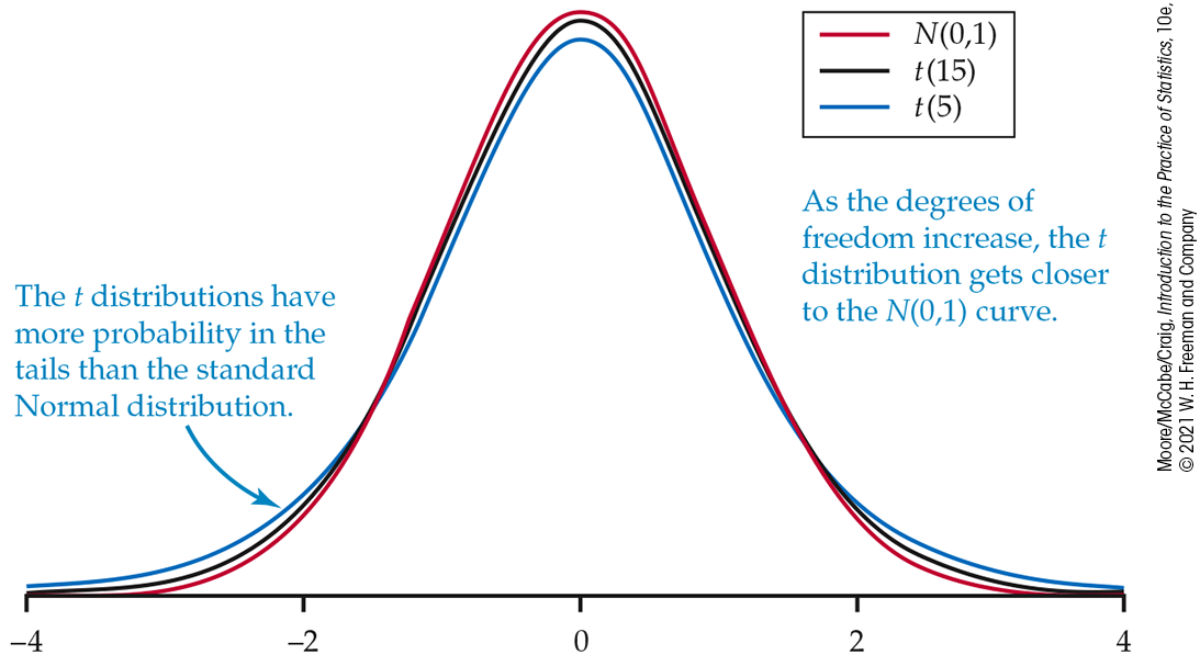
Figure 7.1 Density curves for the standard Normal, t(5), and t(15) distributions. All are symmetric, with center 0.
This greater spread is due to the extra variability caused by
substituting the random variable s for the fixed parameter
Check-in
-
7.1 Two-bedroom apartment rates. Zillow.com contains several hundred postings for two-bedroom apartments in your city. You choose 16 at random and calculate a mean monthly rent of $906 and a standard deviation of $276.
What is the standard error of the mean?
-
What are the degrees of freedom for the one-sample t statistic?
-
7.2 Changing the sample size. Refer to the previous Check-in question. Suppose that instead of having an SRS of 16, you sampled 25 postings.
-
Would you expect the standard error of the mean to be larger or smaller in this case? Explain your answer.
-
State why you can’t be certain that the standard error for this new SRS will be larger or smaller.
-
With the t distributions to help us, we can now analyze an SRS
from a Normal population with unknown
One-sample t confidence interval
The one-sample t confidence interval is similar in both
reasoning and computational detail to the z confidence interval
of Chapter 6. There,
the margin of error for the population mean was
Example 7.1 Average delivery time for robot service.
![]()
Your university recently launched robot food delivery services that
works in conjunction with your meal plan. An advertisement states
that you can order food and drinks to be delivered anywhere on
campus, within minutes.1
You decide to investigate this claim and record the delivery times
for your weekday lunch orders from Cosi. Let’s construct a 95%
confidence interval for the average delivery time (in minutes) from
Cosi to your dormitory based on the following
The sample mean is
and the standard deviation is
with degrees of freedom
|
|
|||
|
|
1.895 | 2.365 | 2.517 |
| C | 0.90 | 0.95 | 0.96 |
From
Table D, we find
We are 95% confident that the average delivery time from Cosi to your dormitory is between 11.1 and 35.1 minutes.
In this example, we have given the actual interval (11.1, 35.1)
minutes as our answer. Sometimes, we prefer to report the mean and
margin of error: the mean time is 23.1 minutes, with a margin of error
of 12.0 minutes. This is a large margin of error in relation to size
of the estimated mean. In
Section 7.3, we will return to this example and discuss determining an
appropriate sample size for a smaller margin of error, such as
Valid interpretation of the t confidence interval in Example 7.1 rests on assumptions that appear reasonable here. First, we assume that our sample of delivery times is an SRS from the population of all weekday delivery times from Cosi to your dormitory. Because your decision to order from Cosi on a weekday is fairly random, this is likely reasonable. If you only ordered from Cosi on Thursdays, generalizing to any weekday may be suspect as the campus foot traffic and robot delivery demands may vary day to day.
We also assume that the distribution of delivery times is Normal. With
only eight observations, this assumption cannot be effectively
checked. We can, however, check if the data suggest a severe departure
from Normality.
Figure 7.2
shows the Normal quantile plot, and we can see that there are no
extreme outliers, and there is no severe skewness. Deciding whether to
use the t procedures for inference about
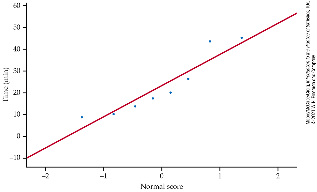
Figure 7.2 Normal quantile plot of the data, Example 7.1.
Check-in
-
7.3 More on apartment rents. Recall Check-in question 7.1 (page 386). Assume that the rents are Normally distributed.
-
Construct a 95% confidence interval for the mean monthly rent of two-bedroom apartments.
-
Can we consider that this interval applies to the mean of all two-bedroom apartment rents in your city? Explain your answer.
-
-
7.4 Finding critical
-
a 90% confidence interval when
-
a 95% confidence interval when
-
a 99% confidence interval when
-
The one-sample t test
Significance tests of the mean
Example 7.2 Significance test for robot delivery service.
![]()
If you were to pick up an order from Cosi, it would take you 15 minutes to walk there and back. Focusing just on the time it takes to get an order, we might want to test whether the average robot delivery time differs from this 15 minutes. Specifically, we want to test
at the 0.05 significance level. Recall that
This means that the sample mean
|
|
||
| p | 0.10 | 0.05 |
|
|
1.415 | 1.895 |
Because the degrees of freedom are
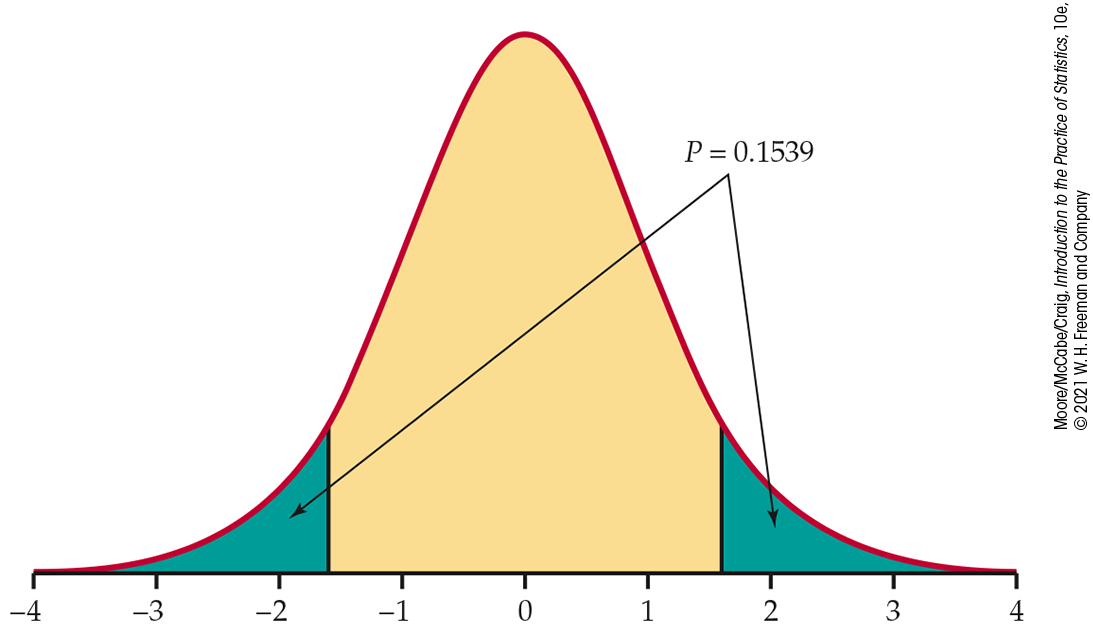
Figure 7.3 Sketch of the P-value calculation, Example 7.2.
Therefore, we conclude that the P-value is between
=T.DIST.2T(1.599,7),
where the first input is the absolute value of the test statistic
and the second input is the degrees of freedom. It gives
These data are compatible with an average of 15.0 minutes. Under
In this example, we tested the null hypothesis
Example 7.3 One-sided test for robot delivery service.
![]()
For the problem described in the previous example, we want to test whether the robot average delivery time is larger than the stated 15.0 minutes. Here we test
versus
The t test statistic does not change:
=T.DIST.RT(1.599,7). Similar to
the two-sided alternative, there is not enough evidence to reject
the null hypothesis in favor of the alternative at the 0.05
significance level.
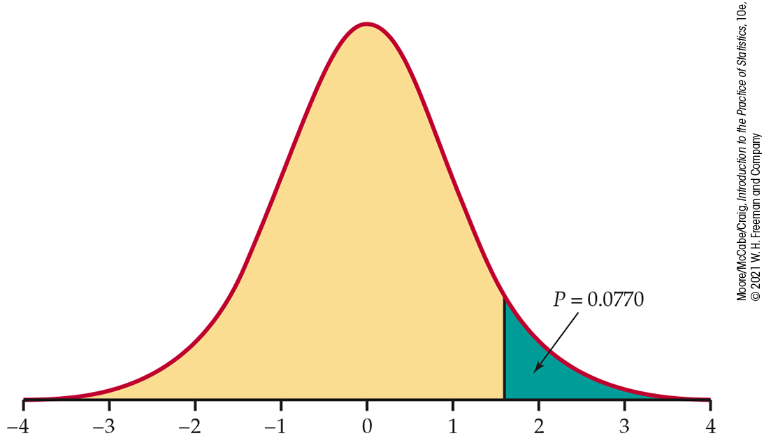
Figure 7.4 Sketch of the P-value calculation, Example 7.3.
For the robot delivery example, our conclusion did not depend on the
choice between one-sided and two-sided alternatives. Sometimes,
however, this choice will affect the conclusion, and so this
choice needs to be made prior to analysis. If in doubt, always use a
two-sided test.
![]() It is wrong to examine the data first and then decide to do a
one-sided test in the direction indicated by the data.
Often, a significant result for a two-sided test can be used to
justify a one-sided test for another sample from the same
population.
It is wrong to examine the data first and then decide to do a
one-sided test in the direction indicated by the data.
Often, a significant result for a two-sided test can be used to
justify a one-sided test for another sample from the same
population.
Check-in
-
7.5 Significant? A two-sided t test for the mean
-
The sample size is 28. Is the test result significant at the 5% level? Explain how you obtained your answer.
-
The sample size is 10. Is the test result significant at the 5% level? Explain how you obtained your answer.
-
Sketch the two t distributions to illustrate your answers.
-
-
7.6 Significance test for apartment rents. Refer to Check-in questions 7.1 (page 386) and 7.3 (page 388). Do the data give good reason to believe that the mean rent of all two-bedroom apartments is greater than $750? State the hypotheses, find the t statistic and its P-value, and state your conclusion using the 5% significance level.
Using software
![]()
For small data sets, such as the one in Example 7.1 (page 387), it is easy to perform the computations for confidence intervals and significance tests with an ordinary calculator and Table D. For larger data sets, however, we prefer to use software.
Example 7.4 Stock portfolio diversification?
![]()
An investor with a stock portfolio worth several hundred thousand dollars sued his broker and brokerage firm because lack of diversification in his portfolio led to poor performance. TABLE 7.1 gives the rates of return for the 39 months that the account was managed by the broker. An arbitration panel compared these returns with the average of the Standard & Poor’s 500-stock index for the same period.2 Let’s do the same using the one-sample t test.
|
|
1.63 |
|
|
|
|
|
|
| 6.82 |
|
|
6.13 | 7.00 |
|
|
|
|
|
|
|
|
|
|
|
1.28 |
|
|
4.34 | 12.22 |
|
|
7.34 | 5.04 |
|
|
|
|
|
12.03 |
|
4.33 | 2.35 |
Consider the 39 monthly returns as a random sample from the
population of possible monthly returns the brokerage firm would
generate during this time period. Are these returns compatible with
a population mean of
Figure 7.5
gives a histogram and summary statistics for these data using JMP.
There are no outliers, and the distribution shows no strong
skewness. Thus, we are reasonably confident that the distribution of
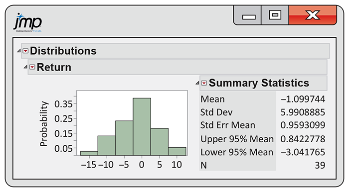
Figure 7.5 Histogram and summary statistics of monthly rates of return for a stock portfolio using JMP, Example 7.4.
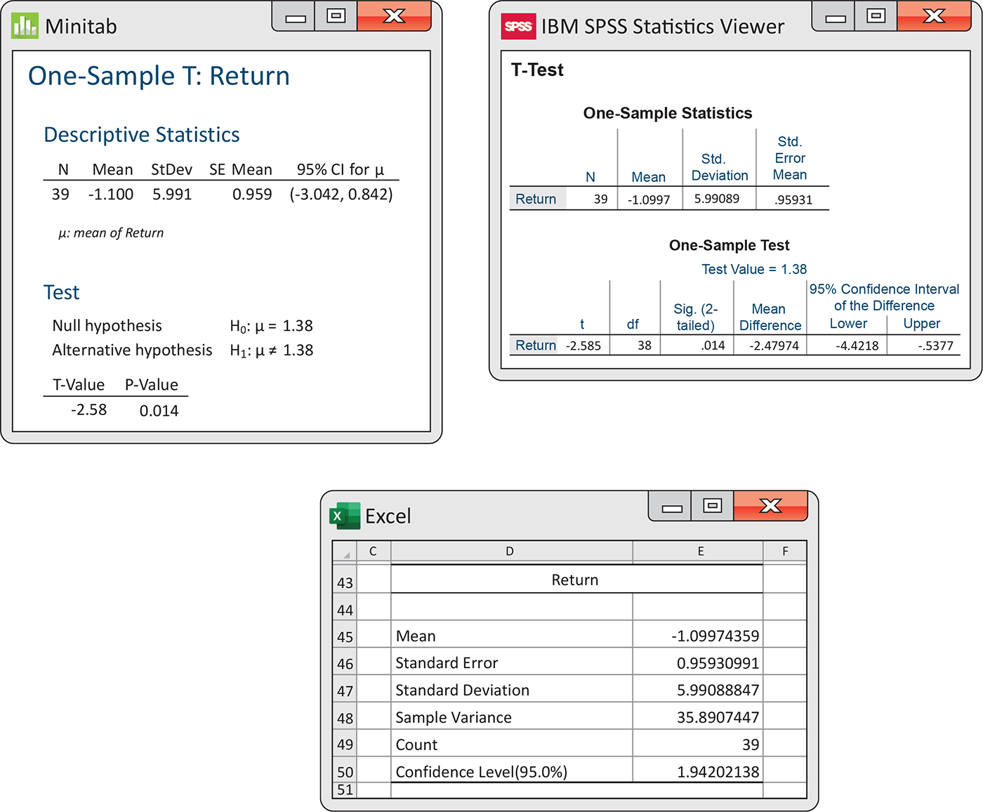
Figure 7.6 Minitab, SPSS, and Excel outputs, Examples 7.4 and 7.5.
Here is one way to report the conclusion: the mean monthly return on
investment for this client’s account was
The hypothesis test in Example 7.4 leads us to conclude that the mean return on the client’s account differs from that of the S&P 500 index. Now let’s assess the return on the client’s account with a confidence interval.
Example 7.5 Estimating the mean monthly return.
![]()
The mean monthly return on the client’s portfolio was
Because the S&P 500 return, 1.38%, falls outside this interval, we
know that
Example 7.6 Estimating the difference from a standard.
![]()
The difference between the mean of the investor’s account and the
S&P 500 is
The assumption that these 39 monthly returns represent an SRS from the population of monthly returns from the brokerage during this time period is certainly debatable. One could also argue that we should not consider the S&P 500 monthly average return as a constant standard. Its return would also vary from month to month. If those monthly returns were available, an alternative analysis would be to compare the average difference between each monthly return for this account and for the S&P 500. This type of comparison is discussed next.
Check-in
-
7.7 Using software to obtain a confidence interval. In Example 7.1 (page 387), we calculated the 95% confidence interval for average delivery time of a delivery robot. Use software to compute this interval and verify that you obtain the same interval.

-
7.8 Using software to perform a significance test. In Example 7.2 (page 389), we tested whether the average delivery time for the robot differs from 15 minutes at the 0.05 significance level. Use software to perform this test and obtain the exact P-value.
Matched pairs t procedures
![]()
The robot delivery problem of Example 7.1 concerns only a single population. We know that comparative studies are usually preferred to single-sample investigations because of the protection they offer against confounding. For that reason, inference about a parameter of a single distribution is less common than comparative inference.
One common comparative design, however, makes use of single-sample procedures. In a matched pairs study, subjects are matched in pairs, and their outcomes are compared within each matched pair. For example, an experiment to compare the interest in two smartphone packages might use pairs of subjects who are the same age, sex, and income level. The experimenter could toss a coin to assign the two packages to the two subjects in each pair. The idea is that matched subjects are more similar than unmatched subjects, so comparing outcomes within each pair is more efficient (i.e., reduces the standard deviation of the estimated difference of treatment means).
Matched pairs are also common when randomization is not possible. For example, one situation calling for matched pairs is when observations are taken on the same subjects under two different conditions. Here is an example.
Example 7.7 The effect of altering a software parameter.
![]()
The MeasureMind® 3D MultiSensor metrology software is used by various companies to measure complex machine parts. As part of a technical review of the software, researchers at GE Healthcare discovered that unchecking one software option reduced measurement time by 10%. This time reduction would help the company’s productivity, provided that the option had no impact on the measurement outcome. To investigate this, the researchers measured 51 parts using the software both with and without this option checked.3 The experimenters tossed a fair coin to decide which measurement (with or without the option) to take first.
TABLE 7.2 gives the measurements (in microns) for the first 20 parts. For analysis, we subtract the measurement with the option on from the measurement with the option off. These differences form a single sample and appear in the “Diff” columns for each part.
| Part | OptionOn | OptionOff | Diff | Part | OptionOn | OptionOff | Diff |
|---|---|---|---|---|---|---|---|
| 1 | 118.63 | 119.01 | 0.38 | 11 | 119.03 | 118.66 |
|
| 2 | 117.34 | 118.51 | 1.17 | 12 | 118.74 | 118.88 | 0.14 |
| 3 | 119.30 | 119.50 | 0.20 | 13 | 117.96 | 118.23 | 0.27 |
| 4 | 119.46 | 118.65 |
|
14 | 118.40 | 118.96 | 0.56 |
| 5 | 118.12 | 118.06 |
|
15 | 118.06 | 118.28 | 0.22 |
| 6 | 117.78 | 118.04 | 0.26 | 16 | 118.69 | 117.46 |
|
| 7 | 119.29 | 119.25 |
|
17 | 118.20 | 118.25 | 0.05 |
| 8 | 120.26 | 118.84 |
|
18 | 119.54 | 120.26 | 0.72 |
| 9 | 118.42 | 117.78 |
|
19 | 118.28 | 120.26 | 1.98 |
| 10 | 119.49 | 119.66 | 0.17 | 20 | 119.13 | 119.15 | 0.02 |
To assess whether there is a difference between the measurements with and without this option, we test
Here,
The 51 differences have
Figure 7.7 shows a histogram and estimated Normal density curve of the differences. The data are reasonably symmetric, with no outliers, so based on the guidelines we discuss next (page 398), we can comfortably use the one-sample t procedures. Remember to always check assumptions before proceeding with statistical inference.
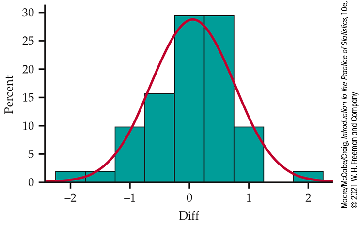
Figure 7.7 Histogram of differences in measurements, Example 7.7.
The one-sample t statistic is
The P-value is found from the t(50) distribution. Remember that the degrees of freedom are 1 less than the sample size.
Table D
shows that 0.52 lies to the left of the first column entry. This
means the P-value is greater than
This result, however, does not fully address the goal of this study.
![]() A lack of statistical significance does not prove the null
hypothesis is true.
If that were the case, we would simply design poor experiments
whenever we wanted to prove the null hypothesis. The more appropriate
method of inference in this setting is to consider
equivalence
testing. With this approach, we try to prove that the mean difference is
within some acceptable region around 0. We can actually perform this
test using a confidence interval.
A lack of statistical significance does not prove the null
hypothesis is true.
If that were the case, we would simply design poor experiments
whenever we wanted to prove the null hypothesis. The more appropriate
method of inference in this setting is to consider
equivalence
testing. With this approach, we try to prove that the mean difference is
within some acceptable region around 0. We can actually perform this
test using a confidence interval.
Example 7.8 Are the two means equivalent?
![]()
Suppose the GE Healthcare researchers state that a mean difference
less than 0.20 micron is not important. To see if the data support a
mean difference within
The standard error is
so the margin of error is
where the critical value
|
|
||
|
|
1.676 | 2.009 |
| C | 90% | 95% |
This interval is not entirely within the
One can also use statistical software to perform an equivalence test. Figure 7.8 shows the Minitab output for Example 7.8. It is common to visually present the test using the confidence interval and the user-specified upper and lower equivalence limits.
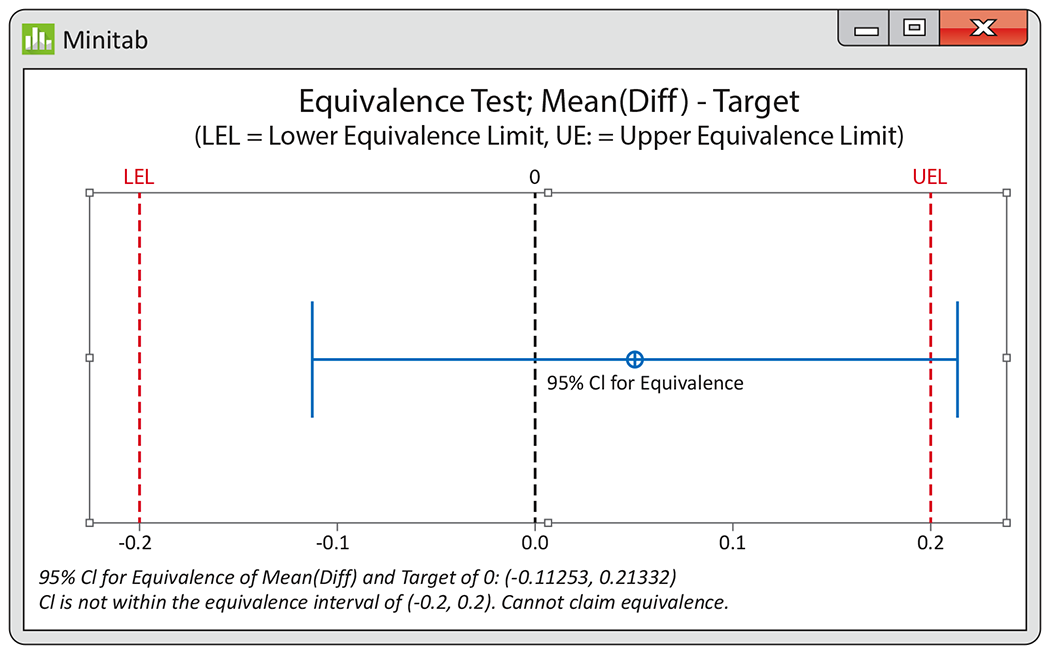
Figure 7.8 Minitab output of the equivalence test, Example 7.8.
Check-in
-
7.9 Female wolf spider mate preferences. As part of a study on factors affecting mate choice, researchers exposed 18 premature female wolf spiders twice a day until maturity to iPod videos of three courting males with average-size tufts. Once mature, each female spider was exposed to two videos, one involving a male with large tufts and the other involving a male with small tufts. The number of receptivity displays by the female toward each male was recorded.4 Explain why a paired t-test is appropriate in this setting.
-
7.10 Cold plasma technology. Cold plasma (CP) technology has been shown to be an effective tool for shelf-life extension of food.5 For it to become widely used, however, CP’s effects on food quality must be understood. Consider the following study, which compared the taste of fruit juice with and without CP treatment. Each juice was rated, by a set of taste experts, using a 0 to 100 scale, with 100 being the highest rating. For each expert, a coin was tossed to see which juice was tasted first.

Expert 1 2 3 4 5 6 7 8 9 10 With CP: 93 65 37 78 89 49 88 55 63 62 Without CP: 92 67 47 79 84 52 80 52 67 69 Is there a difference in taste? State the appropriate hypotheses and carry out a matched pairs t test using
-
7.11 Are the means equivalent? Refer to the previous Check-in question. Other research has suggested that a difference of
Robustness of the t procedures
The matched pairs t procedures and the test of equivalence use one-sample t confidence intervals and significance tests for differences. They are, therefore, based on an assumption that the population of differences has a Normal distribution. For the histogram of the 51 differences in Example 7.7 shown in Figure 7.7 (page 395), the data appear to be slightly skewed. Does this slight non-Normality suggest that we should not use the t procedures for these data?
All inference procedures are based on some conditions, such as Normality. Procedures that are not strongly affected by violations of a condition are called robust. Robust procedures are very useful in statistical practice because they can be used over a wide range of conditions with good performance.
The condition that the population is Normal rules out outliers, so the
presence of outliers shows that this assumption is not valid. The
t procedures are not robust against outliers because
Fortunately, the t procedures are quite robust against non-Normality of the population, particularly when the sample size is large. This is true because:
-
The central limit theorem says that the sampling distribution of the sample mean
-
As the sample size n grows, the sample standard deviation s will be an accurate estimate of
![]() To convince yourself of this fact, use the
Distribution of the One-Sample t Statistic applet to
study the sampling distribution of the one-sample t statistic.
From one of three population distributions, 10,000 SRSs of a
user-specified sample size n are generated, and a histogram of
the t statistics is constructed. You can then compare this
estimated sampling distribution with the
To convince yourself of this fact, use the
Distribution of the One-Sample t Statistic applet to
study the sampling distribution of the one-sample t statistic.
From one of three population distributions, 10,000 SRSs of a
user-specified sample size n are generated, and a histogram of
the t statistics is constructed. You can then compare this
estimated sampling distribution with the
To assess whether the t procedures can be used in practice, a
Normal quantile plot, stemplot, or boxplot can be used to check for
skewness and outliers. For most purposes, the one-sample
t procedures can be safely used when
- Sample size less than 15: Use t procedures if the data are close to Normal. If the data are clearly non-Normal or if outliers are present, do not use t.
- Sample size at least 15 and less than 40: Use the t procedures except in the presence of outliers or strong skewness.
-
Large samples (
For the robot delivery study in
Example 7.1,
there are only
Check-in
-
7.12 t procedures for average business start time? Consider the data from Example 1.19 (page 26). Would you be comfortable using the t procedures for inference on the average business start time? Explain your answer.

-
7.13 t procedures for a larger sample? Now consider the data for all 187 countries as an SRS from the population of potential start times. Would you be comfortable applying the t procedures in this case? Explain your answer.

Inference for non-normal populations
So what do you do when the populations are clearly non-Normal and you are not comfortable assuming that the sample size is large enough to rely on the robustness of the t procedures? Our recommendation is to consult an expert. There are three general strategies, but each quickly moves beyond the basic practice of statistics:
- In some cases, a distribution other than a Normal distribution describes the data well. There are many non-Normal models for data, and inference procedures for these models are available.
- Because skewness is the chief barrier to the use of t procedures on data without outliers, you can attempt to transform skewed data so that the distribution is symmetric and as close to Normal as possible. Confidence levels and P-values from the t procedures applied to the transformed data will be quite accurate for even moderate sample sizes. Methods are generally available for transforming the results back to the original scale.
- Use a distribution-free inference procedure. Such procedures do not assume that the population distribution has any specific form, such as Normal. Distribution-free procedures are often called nonparametric procedures. Chapter 15 discusses several of these procedures.
We emphasize procedures based on Normal distributions because they are the most common in practice, because their robustness makes them widely useful, and (most importantly) because we are first of all concerned with understanding the principles of inference. Nonetheless, it is helpful to illustrate by example a couple of these approaches—in particular, the use of a transformation and the use of a simple distribution-free procedure.
Transforming data
When the distribution of a variable is skewed, it often happens that a transformation results in a variable whose distribution is symmetric and even close to Normal. The most common transformation is the logarithm, or log. The logarithm tends to pull in the right tail of a distribution. For example, the data 2, 3, 4, 20 show an outlier in the right tail. Their natural logarithms 0.30, 0.48, 0.60, 1.30 are much less skewed. Taking logarithms is a possible remedy for right-skewness. Instead of analyzing values of the original variable X, we compute their logarithms and analyze the values of X.
Example 7.9 Length of songs in a Spotify library.
![]()

TABLE 7.3
presents data on the length (in seconds) of songs found in a
“Liked Songs” Spotify library. The library contained a total of
8173 songs, and 50 songs were randomly selected using the “shuffle
play” option.7
We would like to give a confidence interval for the average song
length
| 240 | 316 | 259 | 46 | 871 | 411 | 1366 |
| 233 | 520 | 239 | 259 | 535 | 213 | 492 |
| 315 | 696 | 181 | 357 | 130 | 373 | 245 |
| 305 | 188 | 398 | 140 | 252 | 331 | 47 |
| 309 | 245 | 69 | 293 | 160 | 245 | 184 |
| 326 | 612 | 474 | 171 | 498 | 484 | 271 |
| 207 | 169 | 171 | 180 | 269 | 297 | 266 |
| 1847 |
A Normal quantile plot of these data (Figure 7.9) shows that the distribution is non-negative and skewed to the right. Even for this clearly skewed distribution, the guidelines suggest that the sample mean of the 50 observations will nonetheless have an approximately Normal sampling distribution. Thus, the t procedures could be used for approximate inference. For more exact inference, we will transform the data so that the distribution is more nearly Normal. Figure 7.10 is a Normal quantile plot of the natural logarithms of the time measurements. The transformed data are very close to Normal, so t procedures will give quite exact results.
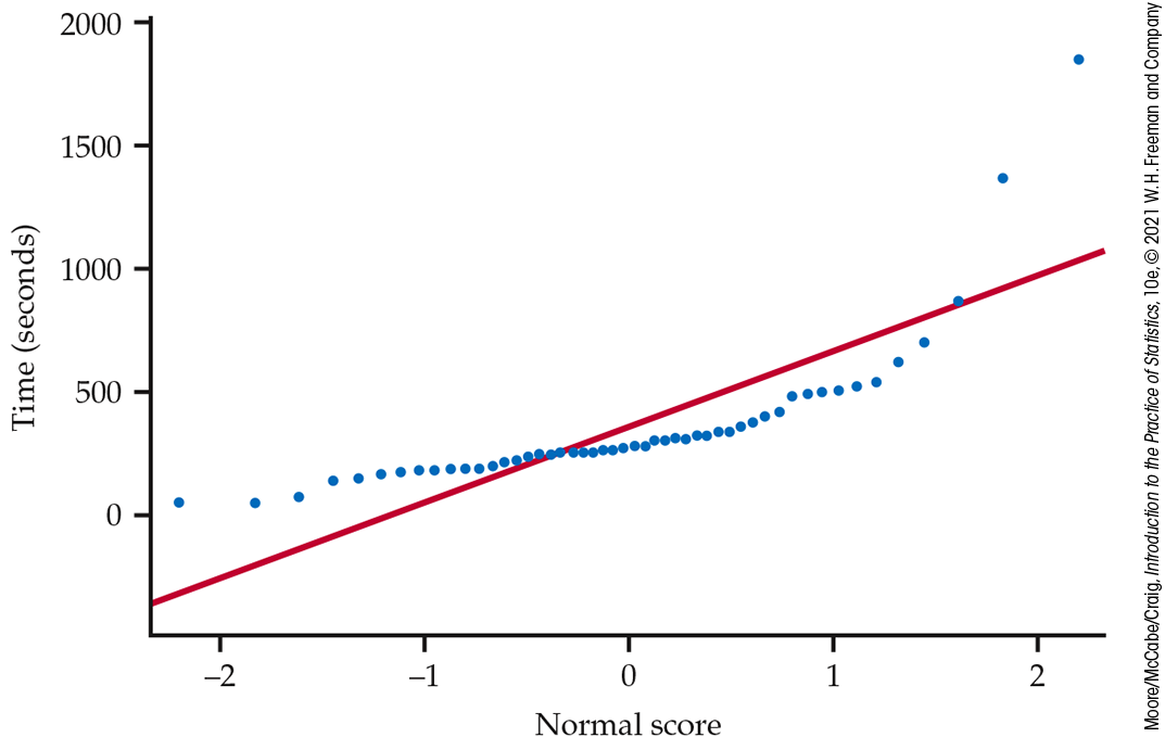
Figure 7.9 Normal quantile plot of audio file length, Example 7.9. This sort of pattern occurs when a distribution is skewed to the right.
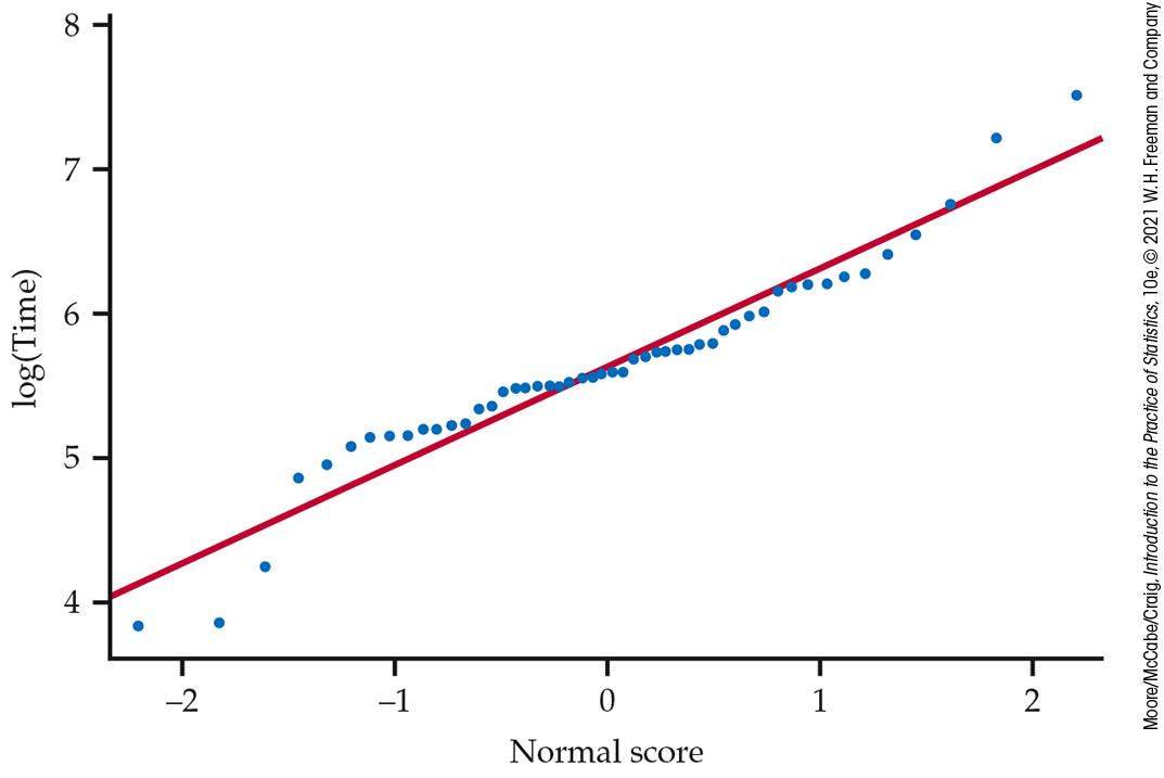
Figure 7.10 Normal quantile plot of the logarithms of the audio file lengths, Example 7.9. This distribution appears approximately Normal.
The application of the t procedures to the transformed data
is straightforward. Call the original length values from
Table 7.3 the
variable X. The transformed data are values of
Example 7.10 Software output of audio length data.
![]()
Analysis of the natural log of the length values in Minitab produces the following output:
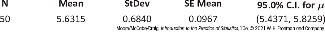
For comparison, the 95% t confidence interval for the
original mean

The advantage of analyzing transformed data is that use of
procedures based on the Normal distributions is better justified,
and the results are more exact. The disadvantage is that a
confidence interval for the mean
Use of a distribution-free procedure
Perhaps the most straightforward way to cope with non-Normal data is to use a distribution-free procedure. As the name indicates, these procedures do not require that the data follow any specific distribution, such as Normal. This gain in generality, however, is not free. First, if the data are close to Normal, distribution-free procedures are generally less powerful than the t test. Second, they don’t quite answer the same question. One-sample distribution-free procedures ask about the population median, as this is a natural measure of population center for a skewed distribution.
The simplest distribution-free procedure, and one of the most useful, is the sign test. The test gets its name from the fact that we look only at the signs of the differences, not their actual values. The following example illustrates this test.
Example 7.11 The effect of altering a software parameter.
![]()
Example 7.7 (page 394) describes an experiment to compare the measurements obtained from two software algorithms. In that example, we used the matched pairs t test on these data, despite some skewness, which makes the P-value only roughly correct. The sign test is based on the following simple observation: of the 51 parts measured, 29 had a larger measurement with the option off, and 22 had a larger measurement with the option on.
To perform a significance test based on these counts, let p be the probability that a randomly chosen part would have a larger measurement with the option turned off. The null hypothesis of “no effect” says that the two measurements on each part are just repeat measurements. Thus, measurement with the option off is equally likely to be larger or smaller than the measurement with the option on. Therefore, we want to test
The 51 parts are independent trials, so the number that had larger
measurements with the option off has the binomial distribution
B(51, 1/2) if
As in Example 7.7, there is not strong evidence that the two measurements are different.
There are several varieties of sign test, all based on counts and
the binomial distribution. The sign test for matched pairs is the
most useful. The null hypothesis of “no effect” is then always
The matched pairs t test in
Example 7.7
tested the hypothesis that the mean of the distribution of
differences is 0. The sign test in
Example 7.11
is, in fact, testing the hypothesis that the median of the
differences is 0. If p is the probability that a difference
is positive, then
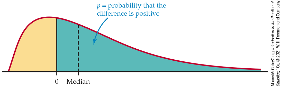
Figure 7.11 Why the sign test tests the median difference: when the median is greater than 0, the probability p of a positive difference is greater than 1/2 and vice versa.
The sign test in Example 7.11 makes no use of the actual scores; it just counts how many parts had a larger measurement with the option off. Any parts that did not have different measurements would be ignored altogether. Because the sign test uses so little of the available information, it is much less powerful than the t test when the population is close to Normal. Chapter 15 describes other distribution-free procedures that are more powerful than the sign test.
Check-in
-
7.14 Sign test for the cold-plasma study. Check-in question 7.10 (page 397) gives data on the taste of fruit juice with and without CP treatment. Is there evidence that the median difference in taste is nonzero? State the hypotheses, carry out the sign test, and report your conclusion.
Example 7.12 A bootstrap confidence interval.
![]()
Consider the eight delivery time measurements (in minutes) in Example 7.1:
We defended the use of the one-sided t confidence interval for an earlier analysis. Let’s now compare those results with the confidence interval constructed using the bootstrap.
This can be done using JMP by right-clicking on the numerical mean
value in the summary statistics produced from the distribution
platform and selecting bootstrap. We decide to collect the
with
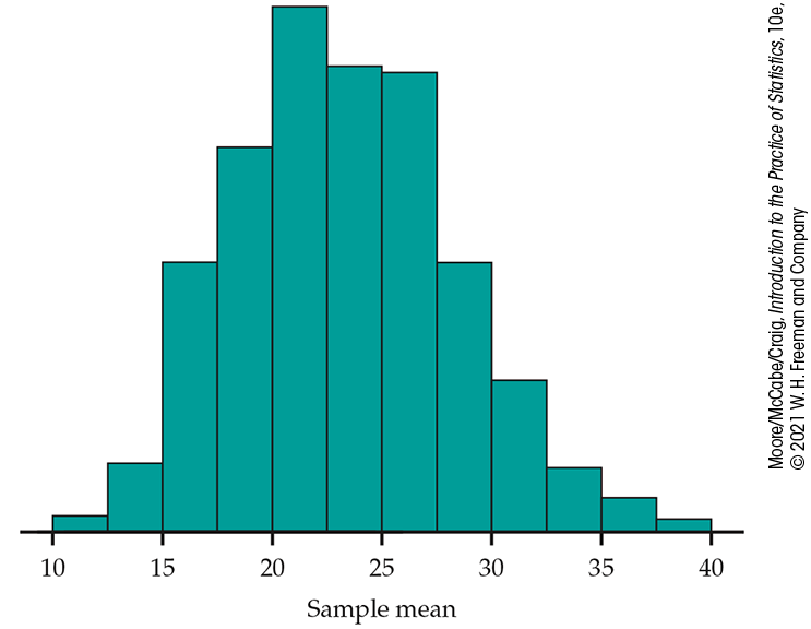
Figure 7.12 Histogram of
Using the middle 95% of the resampled
Section 7.1 SUMMARY
-
Significance tests and confidence intervals for the mean
-
The standard error of
-
The standardized sample mean, or one-sample z statistic,
has the N(0, 1) distribution. If the standard deviation
has the t distribution with
-
There is a t distribution for every positive degrees of freedom k. All are symmetric distributions similar in shape to Normal distributions. The t(k) distribution approaches the N(0, 1) distribution as k increases.
-
The level C margin of error of
where
-
A level C confidence interval for
-
Significance tests for
-
A matched pairs analysis is needed when subjects or experimental units are matched in pairs or when there are two measurements on each individual or experimental unit and the question of interest concerns the difference between the two measurements.
-
The one-sample t procedures are used to analyze matched pairs data by first taking the differences within the matched pairs to produce a single sample of differences.
-
One-sample equivalence testing assesses whether a population mean
-
The t procedures are relatively robust against non-Normal populations. The t procedures are useful for non-Normal data when
-
The sign test is a distribution-free procedure because it uses probability calculations that are correct for a wide range of population distributions.
-
The sign test for “no treatment effect” in matched pairs counts the number of positive differences. The P-value is computed from the B(n, 1/2) distribution, where n is the number of nonzero differences. The sign test is less powerful than the t test in cases where use of the t test is justified.
Section 7.1 EXERCISES
-
7.1 What’s wrong? For each of the following statements, explain what is wrong and why.
-
The degrees of freedom for the one-sample t statistic is
-
The margin of error for the population mean
-
The P-value in a one-sample equivalence test quantifies the evidence provided by the data that
-
A matched pairs analysis is needed whenever you have a study with two treatment conditions.
-
-
7.2 What’s wrong? For each of the following statements, explain what is wrong and why.
-
As the degrees of freedom k decrease, the t distribution density curve gets closer to the N(0, 1) curve.
-
The standard error of the sample mean is
-
A researcher wants to test
-
The 95% margin of error for the mean
-
-
7.3 Finding the critical value
-
A 95% confidence interval based on
-
A 95% confidence interval from an SRS of 26 observations.
-
A 90% confidence interval from a sample of size 26.
-
These cases illustrate how the size of the margin of error depends upon the confidence level and the sample size. Summarize these relationships.
-
-
7.4 Distribution of the t statistic. Assume a sample size of
-
7.5 More on the distribution of the t statistic. Repeat the previous exercise for the two situations where the alternative is one-sided.
-
7.6 A one-sample t test. The one-sample t statistic for testing
from a sample of
-
What are the degrees of freedom for this statistic?
-
Give the two critical values
-
Between what two values does the P-value of the test fall?
-
Is the value
-
If you have software available, find the exact P-value.
-
-
7.7 Another one-sample t test. The one-sample t statistic for testing
from a sample of
-
What are the degrees of freedom for t?
-
Locate the two critical values
-
Between what two values does the P-value of the test fall?
-
Is the value
-
If you have software available, find the exact P-value.
-
-
7.8 A final one-sample t test. The one-sample t statistic for testing
based on
-
What are the degrees of freedom for this statistic?
-
Between what two values does the P-value of the test fall?
-
If you have software available, find the exact P-value.
-
-
7.9 Margin of error. For each of the following situations, compute the 95% margin of error for the population mean
-
An SRS of
-
An SRS of
-
An SRS of
-
-
7.10 Business bankruptcies in Canada. Business bankruptcies in Canada are monitored by the Office of the Superintendent of Bankruptcy Canada (OSB).10 Included in each report are the assets and liabilities the company declared at the time of the bankruptcy filing. A study is based on a random sample of 75 bankruptcy reports filed during the year. The average debt (liabilities minus assets) is $5.32 million, with a standard deviation of $5.87 million.
-
Construct a 95% one-sample t confidence interval for the average debt of Canadian companies filing bankruptcy reports this year.
-
For this sample of companies, debt is positive, and the sample standard deviation is larger than the sample mean. This suggests the debt distribution is right skewed. Provide a defense for using the t confidence interval in this case.
-
-
7.11 Fuel economy. Although the Environmental Protection Agency (EPA) establishes the tests to determine the fuel economy of new cars, it often does not perform them. Instead, the test protocols are given to the car companies, and the companies perform the tests themselves. To keep the industry honest, the EPA runs some audits each year. Recently, the EPA announced that Audi and Volkswagen must lower their fuel economy estimates for some models.11 Here are some city miles per gallon (mpg) values for one of the models the EPA investigated:

18.0 15.7 15.8 18.0 18.5 19.8 20.2 20.4 16.9 18.3 19.8 17.2 16.7 17.7 19.5 18.0 Give a 95% confidence interval for
-
7.12 Testing the sticker information. Refer to the previous exercise. The vehicle sticker information for this model stated a city average of 19 mpg. Are these mpg values consistent with the vehicle sticker? Perform a significance test using the 0.05 significance level. Be sure to specify the hypotheses, the test statistic, the P-value, and your conclusion.
-
7.13 Uber driver earnings. On its blog back in 2014, Uber posted a scatterplot using a sample of several thousand drivers in New York City. The plot showed each driver’s average net earnings per hour versus the number of hours worked.12 Here is a sample of earnings (dollars) for 27 drivers working 40 hours a week.

26.25 33.51 43.91 31.91 31.78 43.37 36.66 31.69 31.25 46.86 35.44 40.30 30.93 37.80 42.44 43.80 49.64 36.79 34.10 37.54 30.93 38.40 37.83 21.73 41.62 26.25 33.51 -
Do you think it is appropriate to use the t methods of this section to compute a 95% confidence interval for the 2014 average earnings per hour of New York City Uber drivers working 40 hours a week? Generate a plot to support your answer.
-
Report the 95% confidence interval for
-
Report the 95% confidence interval for the average annual earnings of New York City Uber drivers working 40 hours a week.
-
According to Uber in 2014, the median wage of an Uber driver working at least 40 hours in New York City is $90,766. Can these data be used to assess this claim? Explain your answer. (Note: Due to an increase in driver supply, these earning rates have dropped substantially since then.)
-
-
7.14 Number of friends on Facebook. To mark Facebook’s 10th birthday, Pew Research surveyed people using Facebook to see what they like and dislike about the site. The survey found that among adult Facebook users, the average number of friends is 338. This distribution takes only integer values, so it is certainly not Normal. It is also highly skewed to the right, with a median of 200 friends.13 Consider the following SRS of

107 246 289 177 155 101 80 461 336 78 463 264 827 180 221 1065 79 691 70 921 126 672 296 60 11 227 84 787 18 82 -
Are these data also heavily skewed? Use graphical methods to examine the distribution. Write a short summary of your findings.
-
Do you think it is appropriate to use the t methods of this section to compute a 95% confidence interval for the mean number of friends that Facebook users at your large university have? Explain why or why not.
-
Compute the sample mean and standard deviation, the standard error of the mean, and the margin of error for 95% confidence.
-
Report the 95% confidence interval for
-
-
7.15 Beer before wine, and you’ll feel fine? Some researchers recently performed a study to investigate the order of beer and wine on hangover intensity.14 The study was run with each participant undergoing both orders of beer and wine with at least a week between sessions. Each session involved drinking the first beverage type until a reaching a breath alcohol concentration (BrAC) of 0.05% and then the other beverage type until a BrAC of 0.11%. The following day, once their BrAC had returned to 0, the participant filled out the Acute Hangover Scale (AHS).
-
Explain why this design is a version of a matched-pairs design.
-
To compare the two orders, the researchers computed the difference in AHS scores
-
-
7.16 Using an app or the Web on a smartphone. The Nielsen Company reports that U.S. residents aged 18 to 34 years spend an average of 2.83 hours per day using an app or the Web on a smartphone.15 You wonder if this it true for students at your large university because you rarely see students not using their smartphones. You collect an SRS of
-
Report the 95% confidence interval for
-
Use this interval to test whether the average time for students at your university is different from the average reported by Nielsen. Use the 5% significance level. Summarize your results.
-
-
7.17 Rudeness and its effect on onlookers. Many believe that an uncivil environment has a negative effect on people. A pair of researchers performed a series of experiments to test whether witnessing rudeness and disrespect affects task performance.16 In one study, 34 participants met in small groups and witnessed the group organizer being rude to a “participant” who showed up late for the group meeting. After the exchange, each participant performed an individual brainstorming task in which he or she was asked to produce as many uses for a brick as possible in five minutes. The mean number of uses was 7.88, with a standard deviation of 2.35.
-
Suppose that prior research has shown that the average number of uses a person can produce in five minutes under normal conditions is 10. Given that the researchers hypothesize that witnessing this rudeness will decrease performance, state the appropriate null and alternative hypotheses.
-
Carry out the significance test using a significance level of 0.05. Give the P-value and state your conclusion.
-
-
7.18 Fuel efficiency t test. Computers in some vehicles calculate various quantities related to performance. One of these is the fuel efficiency, or gas mileage, usually expressed as miles per gallon (mpg). For one vehicle equipped in this way, the miles per gallon were recorded each time the gas tank was filled, and the computer was then reset.17 Here are the mpg values for a random sample of 20 of these records:

41.5 50.7 36.6 37.3 34.2 45.0 48.0 43.2 47.7 42.2 43.2 44.6 48.4 46.4 46.8 39.2 37.3 43.5 44.3 43.3 -
Describe the distribution using graphical methods. Is it appropriate to analyze these data using methods based on Normal distributions? Explain why or why not.
-
Find the mean, standard deviation, standard error, and margin of error for 95% confidence.
-
Report the 95% confidence interval for
-
-
7.19 Tree diameter confidence interval. A study of 584 longleaf pine trees in the Wade Tract in Thomas County, Georgia, is described in Example 6.1 (page 329). For each tree in the tract, the researchers measured the diameter at breast height (DBH). This is the diameter of the tree at a height of 4.5 feet, and the units are centimeters (cm). Only trees with DBH greater than 1.5 cm were sampled. Here are the diameters of a random sample of 40 of these trees:

10.5 13.3 26.0 18.3 52.2 9.2 26.1 17.6 40.5 31.8 47.2 11.4 2.7 69.3 44.4 16.9 35.7 5.4 44.2 2.2 4.3 7.8 38.1 2.2 11.4 51.5 4.9 39.7 32.6 51.8 43.6 2.3 44.6 31.5 40.3 22.3 43.3 37.5 29.1 27.9 -
Use a histogram or stemplot and a boxplot to examine the distribution of DBHs. Include a Normal quantile plot if you have the necessary software. Write a careful description of the distribution.
-
Is it appropriate to use the methods of this section to find a 95% confidence interval for the mean DBH of all trees in the Wade Tract? Explain why or why not.
-
Report the mean with the margin of error and the confidence interval. Write a short summary describing the meaning of the confidence interval.
-
Do you think these results would apply to other similar trees in the same area? Give reasons for your answer.
-
-
7.20 Nutritional intake among Canadian high-performance male athletes. Recall Exercise 6.44 (page 366). For one part of the study,
-
State the appropriate
-
Carry out the test, give the P-value, and state your conclusion.
-
Construct a 95% confidence interval for the average deficiency in caloric intake.
-
-
7.21 Corn seed prices. The U.S. Department of Agriculture (USDA) uses sample surveys to obtain important economic estimates. One USDA pilot study estimated from a sample of 30 farms the amount a farmer will pay per planted acre of corn. The mean price was reported as $674.96 with a standard error of $17.19. Give a 95% confidence interval for the amount a farmer will pay per planted acre of corn.18
-
7.22 Stress levels in parents of children with ADHD. In a study of parents who have children with attention-deficit/hyperactivity disorder (ADHD), parents were asked to rate their overall stress level using the Parental Stress Scale (PSS).19 This scale has 18 items that contain statements regarding both positive and negative aspects of parenthood. Respondents are asked to rate their agreement with each statement using a five-point scale
-
Do you think that these data are approximately Normally distributed? Explain why or why not.
-
Is it appropriate to use the methods of this section to compute a 90% confidence interval? Explain why or why not.
-
Find the 90% margin of error and the corresponding confidence interval. Write a sentence explaining the interval and the meaning of the 90% confidence level.
-
To recruit parents for the study, the researchers visited a psychiatric outpatient service in Rohtak, India, and selected 50 consecutive families who met the inclusion and exclusion criteria. To what extent do you think the results can be generalized to all parents with children who have ADHD in India or in other locations around the world?
-
-
7.23 Are the parents feeling extreme stress? Refer to the previous exercise. The researchers considered a score greater than 45 to represent extreme stress. Is there evidence that the average stress level for the parents in this study is above this level? Perform a test of significance using
-
7.24 Potential insurance fraud? Insurance adjusters are concerned about the high estimates they are receiving from Jocko’s Garage. To see if the estimates are unreasonably high, each of 10 damaged cars was taken to Jocko’s and to another garage, and the estimates (in dollars) were recorded. Here are the results:

Car 1 2 3 4 5 Jocko’s 1410 1550 1250 1300 900 Other 1250 1300 1250 1200 950 Car 6 7 8 9 10 Jocko’s 1520 1750 3600 2250 2840 Other 1575 1600 3380 2125 2600 -
For each car, subtract the estimate of the other garage from Jocko’s estimate. Find the mean and the standard deviation for this difference.
-
Test the null hypothesis that there is no difference between the estimates of the two garages. Be sure to specify the null and alternative hypotheses, the test statistic with degrees of freedom, and the P-value. What do you conclude using the 0.05 significance level?
-
Construct a 95% confidence interval for the difference in estimates.
-
The insurance company is considering seeking repayment from 1000 claims filed with Jocko’s last year. Using your answer to part (c), what repayment would you recommend the insurance company seek? Explain your answer.
-
-
7.25 Fuel efficiency comparison t test. Refer to Exercise 7.18. In addition to the computer calculating miles per gallon, the driver also recorded the miles per gallon by dividing the miles driven by the number of gallons at fill-up. The driver wants to determine if these calculations are different.

Fill-up 1 2 3 4 5 6 7 8 9 10 Computer 41.5 50.7 36.6 37.3 34.2 45.0 48.0 43.2 47.7 42.2 Driver 36.5 44.2 37.2 35.6 30.5 40.5 40.0 41.0 42.8 39.2 Fill-up 11 12 13 14 15 16 17 18 19 20 Computer 43.2 44.6 48.4 46.4 46.8 39.2 37.3 43.5 44.3 43.3 Driver 38.8 44.5 45.4 45.3 45.7 34.2 35.2 39.8 44.9 47.5 -
State the appropriate
-
Carry out the test using a significance level of 0.05. Give the P-value and then interpret the result.
-
-
7.26 Counts of picks in a one-pound bag. A guitar supply company must maintain strict oversight on the number of picks it packages for sale to customers. The company’s current advertisement specifies between 900 and 1000 picks in every bag. An SRS of 36 one-pound bags of picks was collected as part of a quality improvement effort within the company. The number of picks in each bag is shown in the following table.

924 925 967 909 959 937 970 936 952 919 965 921 913 886 956 962 916 945 957 912 961 950 923 935 969 916 952 917 977 940 924 957 920 986 895 923 -
Create (i) a histogram or stemplot, (ii) a boxplot, and (iii) a Normal quantile plot of these counts. Write a careful description of the distribution. Make sure to note any outliers and comment on the skewness and Normality of the data.
-
Based on your observations in part (a), is it appropriate to analyze these data using the t procedures? Briefly explain your response.
-
Find the mean, the standard deviation, and the standard error of the mean for this sample.
-
Calculate the 90% confidence interval for the mean number of picks in a one-pound bag.
-
-
7.27 Significance test for the average number of picks. Refer to the previous exercise.
-
Do these data provide evidence that the average number of picks in a one-pound bag is greater than 925? Using a significance level of 5%, state your hypotheses, the P-value, and your conclusions.
-
Do these data provide evidence that the average number of picks in a one-pound bag is greater than 935? Using a significance level of 5%, state your hypotheses, the P-value, and your conclusion.
-
Explain the relationship between your conclusions in parts (a) and (b) and the 90% confidence interval calculated in the previous problem.
-
-
7.28 A customer satisfaction survey. Many organizations are doing surveys to determine the satisfaction of their customers. Attitudes toward various aspects of campus life were the subject of one such study conducted at Purdue University. Each item was rated on a 1 to 5 scale, with 5 being the highest rating. The average response of 1378 first-year students to “Feeling welcomed at Purdue” was 3.89, with a standard deviation of 1.19. Assuming that the respondents are an SRS, give a 95% confidence interval for the mean of all first-year students.
-
7.29 Comparing operators of a DXA machine. Dual-energy X-ray absorptiometry (DXA) is a technique for measuring bone health. One of the most common measures is total body bone mineral content (TBBMC). A highly skilled operator is required to take the measurements. Recently, a new DXA machine was purchased by a research lab, and two operators were trained to take the measurements. TBBMC for eight subjects was measured by both operators.20 The units are grams (g). A comparison of the means for the two operators provides a check on the training they received and allows us to determine if one of the operators is producing measurements that are consistently higher than the other. Here are the data:

Subject Operator 1 2 3 4 5 6 7 8 1 1.328 1.342 1.075 1.228 0.939 1.004 1.178 1.286 2 1.323 1.322 1.073 1.233 0.934 1.019 1.184 1.304 -
Take the difference between the TBBMC recorded for Operator 1 and the TBBMC for Operator 2. Describe the distribution of these differences. Is it appropriate to analyze these data using the t methods? Explain why or why not.
-
Use a significance test to examine the null hypothesis that the two operators have the same mean. Be sure to give the test statistic with its degrees of freedom, the P-value, and your conclusion.
-
The sample here is rather small, so we may not have much power to detect differences of interest. Use a 95% confidence interval to provide a range of differences that are compatible with these data.
-
The eight subjects used for this comparison were not a random sample. In fact, they were friends of the researchers whose ages and weights were similar to those of the types of people who would be measured with this DXA machine. Comment on the appropriateness of this procedure for selecting a sample and discuss any consequences regarding the interpretation of the significance-testing and confidence interval results.
-
-
7.30 Equivalence of paper and computer-based questionnaires. Computers are commonly used to complete questionnaires because of the increased efficiency of data collection and reduction in coding errors. Studies, however, have shown that questionnaire format can influence responses, especially for items of a sensitive nature.21 Consider the data for the small study below, comparing paper and computer survey formats of a self-report measure of mental health. Each participant completed both forms on adjacent days with the order determined by a flip of a coin.

Subject Paper Computer Diff Subject Paper Computer Diff 1 5 2 3 11 6 5 1 2 4 3 1 12 5 5 0 3 4 4 0 13 3 7 4 7 8 14 3 6 5 4 5 15 4 4 0 6 6 7 16 2 3 7 4 3 1 17 7 10 8 6 8 18 8 7 1 9 6 5 1 19 4 6 10 2 3 20 6 8 -
Explain to someone unfamiliar with statistics why this experiment is a matched pairs design.
-
The measure involves 10 items and produces a whole number score ranging between 0 and 20. Do you think it is appropriate to use the t procedures on the difference in survey scores? Explain your answer.
-
Perform an equivalence test at the 0.05 level using the limits
-
-
7.31 Sign test for potential insurance fraud. The differences in the repair estimates in Exercise 7.24 can also be analyzed using a sign test. Set up the appropriate null and alternative hypotheses, carry out the test, and summarize the results. How do these results compare with those that you obtained in Exercise 7.24?
-
7.32 Sign test for the comparison of operators. The differences in the TBBMC measures in Exercise 7.29 can also be analyzed using a sign test. Set up the appropriate null and alternative hypotheses, carry out the test, and summarize the results. How do these results compare with those that you obtained in Exercise 7.29?
-
7.33 Sign test for fuel efficiency comparison. Use the sign test to assess whether the computer calculates a higher mpg than the driver in Exercise 7.25. State the hypotheses, give the P-value using the binomial table (Table C), and report your conclusion.
-
7.34 Insulation study. A manufacturer of electric motors tests insulation at a high temperature
The small sample size makes judgment from the data difficult, but engineering experience suggests that the logarithm of the failure time will have a Normal distribution. Take the logarithms of the five observations and use t procedures to give a 90% confidence interval for the mean of the log failure time for insulation of this type.