Chapter 10 EXERCISES
-
10.28 School budget and number of students. Suppose that there is a linear relationship between the number of students x in a school system and the annual budget y. Write a population regression model to describe this relationship.
-
Which parameter in your model is the fixed cost in the budget (for example, the salary of the principals and some administrative costs) that does not change as x increases?
-
Which parameter in your model shows how total cost changes when there are more students in the system? Do you expect this number to be greater than 0 or less than 0?
-
Actual data from various school systems will not fit a straight line exactly. What term in your model allows variation among schools of the same size x?
-
-
10.29 Interpreting a residual plot. Figure 10.18 shows four plots of residuals versus x. For each plot, comment on the regression model conditions necessary for inference. Which plots suggest a reasonable fit to the linear regression model?
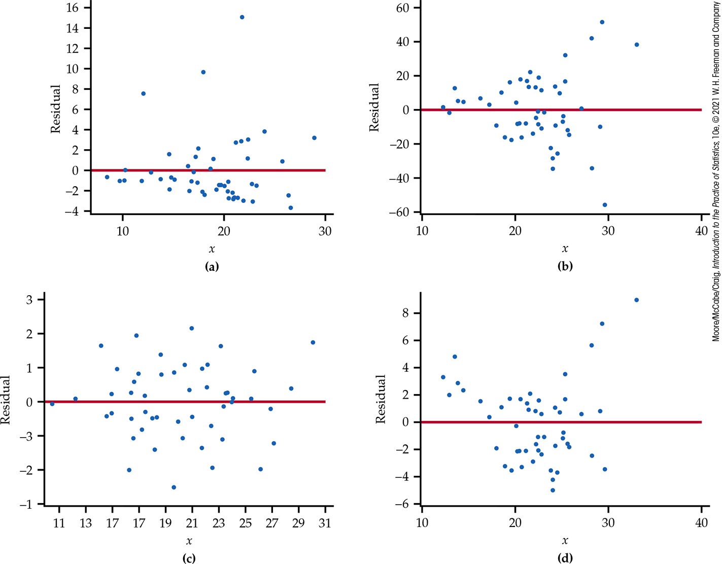
Figure 10.18 Four plots of residual versus x, Exercise 10.29.
-
10.30 The relationship between cell phone use and academic performance. College students are the most rapid adopters of cell phone technology. They use the phone to surf the Internet, watch videos, listen to music, email, and play video games. Because a cell phone is almost always nearby, researchers have begun studying the relationship between cell phone use and various attitudes and behaviors. In one study, researchers assessed the relationship between cell phone use (CPU), cumulative GPA, anxiety, and general life satisfaction (GLS) among 496 students.16
-
Participants were undergraduates from a large midwestern university. They were recruited during class time from courses in sociology, general biology, American politics, human nutrition, and world history. The researchers argued that these courses attracted students from many majors. To participate, students had to consent to have their GPA retrieved. What do you think about this recruitment process? Can we feel comfortable assuming that this is an SRS from the population of undergraduates? Write a short summary of your opinions.
-
The following table summarizes the pairwise correlations among the four variables. For each pair of variables, test the null hypothesis that the correlation is zero. Make sure to state the test statistic, degrees of freedom, and P-value.
GPA Anxiety GLS CPU 0.096 0.012 GPA 0.004 0.207 Anxiety - Write a short paragraph that summarizes your findings.
-
-
10.31 Temperature and academic performance. Does temperature affect academic performance? If yes, does the relationship vary by sex? To study these questions, researchers from Berlin, Germany, divided 543 students into 24 sessions. In each session, students were presented with 50 similar arithmetic problems and given 5 minutes to complete as many as possible. (They were monetarily rewarded for the number of correct answers.) The sessions varied only in terms of the room temperature, which ranged from 16.19 to 32.57°C.17 Although the number of male and female students varied across sessions, let’s look at the relationship between each session’s room temperature (Temp) and the average number of correct answers by sex (Mave and Fave).

-
Make a scatterplot of Mave versus Temp. Describe the relationship.
-
Find the equation of the least-squares regression line for predicting Mave based on the room temperature and add this line to your scatterplot.
-
What is
-
Check the conditions that must be approximately met for inference. Provide a set of plots and any concerns you have.
-
Assuming that inference is appropriate, is there significant evidence that temperature is associated with performance? State the hypotheses, give a test statistic and P-value, and summarize your conclusion.
-
-
10.32 Temperature and academic performance, continued. Refer to the previous exercise. Repeat parts (a)–(e) using the female average score, Fave, as the response variable.
-
10.33 Interpreting the results. Refer to the previous two exercises. You are a math teacher whose pay raise is based on your students’ academic performance. Suppose your class has 40 students, 20 of each sex. Explain how you might use the model results of the previous two exercises to determine an ideal room temperature for your classroom.
-
10.34 Public university tuition: 2014 versus 2018. TABLE 10.2 shows the in-state undergraduate tuition in 2014 and 2018 for 33 public universities.18

Table 10.2 In-state tuition and fees (in dollars) for 33 public universities
University Year2014 Year2018 University Year2014 Year2018 University Year2014 Year2018 Penn State 17,502 18,454 Ohio State 10,037 10,726 Texas 9798 10,606 Pittsburgh 17,772 19,080 Virginia 12,998 17,564 Nebraska 8070 9154 Michigan 13,486 15,262 Cal-Davis 15,589 14,463 Iowa 8079 9267 Rutgers 14,297 14,974 Cal-Berkeley 12,972 14,184 Colorado 10,789 12,532 Michigan State 13,813 14,460 Cal-Irvine 14,757 15,614 Iowa State 7731 8988 Maryland 9427 10,595 Purdue 10,002 9992 North Carolina 8346 8987 Illinois 15,020 15,094 Cal-San Diego 13,456 14,199 Kansas 10,448 11,148 Minnesota 13,626 14,693 Oregon 9918 11,898 Arizona 10,957 12,487 Missouri 11,021 12,055 Wisconsin 10,410 10,555 Florida 6313 6381 Buffalo 8871 10,099 Washington 12,394 11,517 Georgia Tech 11,394 12,424 Indiana 10,388 10,681 UCLA 13,029 13,774 Texas A&M 9179 10,968 -
Plot the data with the 2014 tuition on the x axis and describe the relationship. Are there any outliers or unusual values? Does a linear relationship between the tuition in 2014 and 2018 seem reasonable?
-
Run the simple linear regression and give the least-squares regression line.
-
Obtain the residuals and plot them versus the 2014 tuition amount. Is there anything unusual in the plot?
-
Construct a Normal quantile plot. Do the residuals appear to be approximately Normal? Explain your answer.
-
Using the results of parts (c) and (d), identify and remove any unusual observations and repeat parts (b)–(d).
-
Compare the two sets of least-squares results. Describe any impact these unusual observations have on the results.
-
-
10.35 More on public university tuition. Refer to the previous exercise. We’ll now move forward with inference using the model fit to the data without the unusual observations identified in part (e) of the previous exercise.
-
Give the null and alternative hypotheses for examining if there is a linear relationship between 2014 and 2018 tuition amounts.
-
Write down the test statistic and P-value for the hypotheses stated in part (a). State your conclusions.
-
What percent of the variability in 2018 tuition is explained by a linear regression model using the 2014 tuition?
-
Construct a 95% confidence interval for the slope. Is there evidence that the slope is significantly different from 1? Explain your answer. (Note: If
-
-
10.36 Even more on public university tuition. Refer to the previous two exercises.
-
The tuition at Skinflint U was $9800 in 2014. What is the predicted tuition in 2018?
-
The tuition at I.O.U. was $17,800 in 2014. What is the predicted tuition in 2018?
-
Discuss the appropriateness of using the fitted equation to predict tuition for each of these universities.
-
If you were to construct 95% prediction intervals for each of these universities, which interval would be wider, and why?
-
-
10.37 Predicting public university tuition: 2008 versus 2018. Refer to Exercise 10.35. The data file also includes the in-state undergraduate tuition for the year 2008.
-
Run the simple linear regression using year 2008 in place of year 2014. What is the least-squares line?
Obtain the residuals and check model assumptions.
-
If you had to choose between the model using 2008 tuition and the model using 2014 tuition, which would you choose? Give reasons for your answers.
-
-
 10.38 Draw the fitted line. Suppose you fit 10
pairs of (x, y) data using least squares. Draw the
fitted line if
10.38 Draw the fitted line. Suppose you fit 10
pairs of (x, y) data using least squares. Draw the
fitted line if
-
10.39 Incentive pay and job performance. In the National Football League (NFL), performance bonuses now account for roughly 25% of player compensation.19 Does tying a player’s salary to performance bonuses result in better individual or team success on the field? Focusing on linebackers, let’s look at the relationship between a player’s end-of-year production rating and the percent of his salary devoted to incentive payments in that same year.

-
Use numerical and graphical methods to describe the two variables. Summarize your results.
-
Both variable distributions are non-Normal. Does this necessarily pose a problem for performing linear regression? Explain.
-
Construct a scatterplot of the data and describe the relationship. Are there any outliers or unusual values? Does a linear relationship between the percent of salary and the player rating seem reasonable? Is it a very strong relationship? Explain your answers.
-
Run a simple linear regression and state the least-squares regression line.
-
Obtain the residuals and assess whether the assumptions for the linear regression analysis are reasonable. Include all plots and numerical summaries used in doing this assessment.
-
-
10.40 Performance bonuses, continued. Refer to the previous exercise.
-
Now run the simple linear regression for the variable’s square root of the performance rating and percent of salary devoted to incentive payments.
-
Obtain the residuals and assess whether the assumptions for the linear regression analysis are reasonable. Include all plots and numerical summaries used in doing this assessment.
-
Construct a 95% confidence interval for the square root increase in rating, given a 1% increase in the percent of salary devoted to incentive payments.
-
Consider the values 0%, 20%, 40%, 60%, and 80% salary devoted to incentives. Compute the predicted rating for this model and for the one in the previous exercise. For the model in this problem, you will need to square the predicted value to get back to the original units.
-
Plot the predicted values versus the percent and connect those values from the same model. For which regions of percent do the predicted values from the two models differ the most?
-
Based on the comparison of regression models (both predicted values and residuals), which model do you prefer? Explain.
-
-
10.41 Studying the residuals. Refer to the previous two exercises. Using the residuals from the model fits in Exercise 10.39 and 10.40, who are the top three players to outperform their bonus percent, and who are the top three players to underperform their bonus percent? Does the choice of response variable, untransformed or transformed, impact this list? If so, which model list do you trust more?
-
10.42 Are female CEOs older? A pair of researchers looked at the age and sex of a large sample of CEOs.20 To investigate the relationship between these two variables, they fit a regression model with age as the response variable and sex as the explanatory variable. The explanatory variable was coded
-
What is the expected age for a male CEO
-
What is the expected age for a female CEO
-
What is the difference in the expected age of female and male CEOs?
-
Relate your answers to parts (a) and (c) to the least-squares estimates
-
The t statistic for testing
-
To compare the average age of male and female CEOs, the researchers could have instead performed a two-sample t test (Chapter 7). Will this regression approach provide the same result? Explain your answer.
-
-
10.43 Gambling and alcohol use by first-year college students. Gambling and alcohol use are problematic behaviors for many college students. One study looked at 908 first-year students from a large northeastern university.21 Each participant was asked to fill out the 10-item Alcohol Use Disorders Identification Test (AUDIT) and a 7-item inventory used in prior gambling research among college students. AUDIT assesses alcohol consumption and other alcohol-related risks and problems. (A higher score means more risks.) A correlation of 0.29 was reported between the frequency of gambling and the AUDIT score.
-
What percent of the variability in AUDIT score is explained by frequency of gambling?
-
Test the null hypothesis that the correlation between the gambling frequency and the AUDIT score is zero.
-
The sample in this study represents 45% of the students contacted for the online study. To what extent do you think these results apply to all first-year students at this university? To what extent do you think these results apply to all first-year students? Give reasons for your answers.
-
-
10.44 Predicting water quality. The index of biotic integrity (IBI) is a measure of the water quality in streams. IBI and land use measures for a collection of streams in the Ozark Highland ecoregion of Arkansas were collected as part of a study.22 TABLE 10.3 gives the data for IBI, the percent of the watershed that was forest, and the area of the watershed, in square kilometers, for streams in the original sample with watershed area less than or equal to 70

-
Use numerical and graphical methods to describe the variable IBI. Do the same for area. Summarize your results.
-
Plot the data and describe the relationship between IBI and area. Are there any outliers or unusual patterns?
-
Give the statistical model for simple linear regression for this problem.
-
State the null and alternative hypotheses for examining the relationship between IBI and area.
-
Run the simple linear regression and summarize the results.
-
Obtain the residuals and plot them versus area. Is there anything unusual in the plot?
-
Do the residuals appear to be approximately Normal? Give reasons for your answer.
-
Do the assumptions for the analysis of these data using the model you gave in part (c) appear to be reasonable? Explain your answer.
-
-
10.45 More on predicting water quality.
The researchers who conducted the study described in the previous
exercise also recorded the percent of the
watershed area that was forest for each of the streams. These data
are also given in
Table 10.3. Analyze
these data using the questions in the previous exercise as a
guide.
Table 10.3 Watershed area
Area Forest IBI Area Forest IBI Area Forest IBI Area Forest IBI Area Forest IBI 21 0 47 29 0 61 31 0 39 32 0 59 34 0 72 34 0 76 49 3 85 52 3 89 2 7 74 70 8 89 6 9 33 28 10 46 21 10 32 59 11 80 69 14 80 47 17 78 8 17 53 8 18 43 58 21 88 54 22 84 10 25 62 57 31 55 18 32 29 19 33 29 39 33 54 49 33 78 9 39 71 5 41 55 14 43 58 9 43 71 23 47 33 31 49 59 18 49 81 16 52 71 21 52 75 32 59 64 10 63 41 26 68 82 9 75 60 54 79 84 12 79 83 21 80 82 27 86 82 23 89 86 26 90 79 16 95 67 26 95 56 26 100 85 28 100 91 -
10.46 Comparing the analyses. In Exercises 10.44 and 10.45, you used two different explanatory variables to predict IBI. Summarize the two analyses and compare the results. If you had to choose between the two explanatory variables for predicting IBI, which one would you prefer? Give reasons for your answer.
-
10.47 How an outlier can affect statistical significance. Consider the data in Table 10.3 and the relationship between IBI and the percent of watershed area that was forest. The relationship between these two variables is almost significant at the 0.05 level. In this exercise you will demonstrate the potential effect of an outlier on statistical significance. Investigate what happens when you decrease the IBI to 0.0 for (1) an observation with 0% forest and (2) an observation with 100% forest. Write a short summary of what you have learned from this exercise.
-
10.48 Predicting water quality for an area of 40
-
Find a 95% confidence interval for the mean response corresponding to an area of 40
-
Find a 95% prediction interval for a future response corresponding to an area of 40
-
Write a short paragraph interpreting the meaning of the intervals in terms of Ozark Highland streams.
-
Do you think that these results can be applied to other streams in Arkansas or in other states? Explain why or why not.
-
-
10.49 Compare the predictions. Refer to Exercise 10.46. Another way to compare analyses is to compare predictions. Consider Case 37 in Table 10.3 (8th row, 2nd column). For this case, the area is 10
-
10.50 CEO pay and gross profits. Publicly traded companies must disclose their workers’ median pay and the compensation ratio between a worker and the company’s CEO. Does this ratio say something about the performance of the company? CNBC collected this ratio and the gross profits per employee from a variety of companies.23

-
Generate a scatterplot of the gross profit per employee (Profit) versus the CEO pay ratio (Ratio). Describe the relationship.
-
To compensate for the severe right-skewness of both variables, take the logarithm of each variable. Generate a scatterplot and describe the relationship between these transformed variables.
-
Fit a simple linear regression for log Profits versus log Ratio.
-
Examine the residuals. Are the model conditions approximately satisfied? Explain your answer.
-
Construct a 95% confidence interval for
-
-
10.51 Leaning Tower of Pisa. The Leaning Tower of Pisa is an architectural wonder. Engineers concerned about the tower’s stability have done extensive studies of its increasing tilt. Measurements of the lean of the tower over time provide much useful information. The following table gives measurements for the years 1975 to 1987. The variable Lean represents the difference between where a point on the tower would be if the tower were straight and where it actually is. The data are coded as tenths of a millimeter in excess of 2.9 meters, so that the 1975 lean, which was 2.9642 meters, appears in the table as 642. Only the last two digits of the year were entered into the computer.24

Year 75 76 77 78 79 80 81 82 83 84 85 86 87 Lean 642 644 656 667 673 688 696 698 713 717 725 742 757 -
Plot the data. Does the trend in lean over time appear to be linear?
-
What is the equation of the least-squares line? What percent of the variation in lean is explained by this line?
-
Give a 99% confidence interval for the average rate of change (tenths of a millimeter per year) of the lean.
-
-
10.52 More on the Leaning Tower of Pisa. Refer to the previous exercise.
-
In 1918 the lean was 2.9071 meters. (The coded value is 71.) Using the least-squares equation for the years 1975 to 1987, calculate a predicted value for the lean in 1918. (Note that you must use the coded value 18 for year.)
-
Although the least-squares line gives an excellent fit to the data for 1975 to 1987, this pattern did not extend back to 1918. Write a short statement explaining why this conclusion follows from the information available. Use numerical and graphical summaries to support your explanation.
-
-
10.53 Predicting the lean in 2021. Refer to the previous two exercises.
-
How would you code the explanatory variable for the year 2021?
-
The engineers working on the Leaning Tower of Pisa were most interested in how much the tower would lean if no corrective action were taken. Use the least-squares equation to predict the tower’s lean in the year 2021. (NOTE: The tower was renovated in 2001 to make sure it would not fall down.)
-
To give a margin of error for the lean in 2021, would you use a confidence interval for a mean response or a prediction interval? Explain your choice.
-
-
10.54 Does a math pretest predict success? Can a pretest on mathematics skills predict success in a statistics course? The 62 students in an introductory statistics class took a pretest at the beginning of the semester. The least-squares regression line for predicting the score y on the final exam from the pretest score x was
-
Test the null hypothesis that there is no linear relationship between the pretest score and the score on the final exam against the two-sided alternative.
-
Would you reject this null hypothesis versus the one-sided alternative that the slope is positive? Explain your answer.
-
-
10.55 Significance test of the correlation. A study reported a correlation
-
10.56 State and college binge drinking. Excessive consumption of alcohol is associated with numerous adverse consequences. In one study, researchers analyzed binge-drinking rates from two national surveys, the Harvard School of Public Health College Alcohol Study (CAS) and the Centers for Disease Control and Prevention’s Behavioral Risk Factor Surveillance System (BRFSS).25 The CAS survey was used to provide an estimate of the college binge-drinking rate in each state, and the BRFSS was used to determine the adult binge-drinking rate in each state. A correlation of 0.43 was reported between these two rates for their sample of
-
Find the equation of the least-squares line for predicting the college binge-drinking rate from the adult binge-drinking rate.
-
Give the results of the significance test for the null hypothesis that the slope is 0. (Hint: What is the relation between this test and the test for a zero correlation?)
-
-
10.57 SAT versus ACT. The SAT and the ACT are the two major standardized tests that colleges use to evaluate candidates. Most students take just one of these tests. However, some students take both. Consider the scores of 60 students who did this. How can we relate the two tests?

-
Plot the data with SAT on the x axis and ACT on the y axis. Describe the overall pattern and any unusual observations.
-
Find the least-squares regression line and draw it on your plot. Give the results of the significance test for the slope.
What is the correlation between the two tests?
-
-
10.58 SAT versus ACT, continued. Refer to the
previous exercise. Find the predicted value of ACT for each
observation in the data set.
-
What is the mean of these predicted values? Compare it with the mean of the ACT scores.
-
Compare the standard deviation of the predicted values with the standard deviation of the actual ACT scores. If least-squares regression is used to predict ACT scores for a large number of students such as these, the average predicted value will be accurate, but the variability of the predicted scores will be too small.
-
Find the SAT score for a student who is 1 standard deviation above the mean
-
Repeat part (c) for a student whose SAT score is 1 standard deviation below the mean
-
What do you conclude from parts (c) and (d)? Perform additional calculations for different z’s, if needed.
-
-
10.59 Matching standardized scores.
Refer to the
previous two exercises. An alternative to the least-squares method
is based on matching standardized scores. Specifically, we set
and solve for y. Let’s use the notation
-
Using the data in the previous exercise, find the values of
-
Plot the data with the least-squares line and the new prediction line.
-
Use the new line to find predicted ACT scores. Find the mean and the standard deviation of these scores. How do they compare with the mean and standard deviation of the ACT scores?
-
-
10.60 Are the results consistent? A researcher surveyed
-
10.61 A mechanistic explanation of popularity. Previous experimental work has suggested that the serotonin system plays an important and causal role in social status. In other words, genes may predispose individuals to be popular/likable. As part of a recent study on adolescents, an experimenter looked at the relationship between the expression of a particular serotonin receptor gene, a person’s “popularity,” and the person’s rule-breaking (RB) behaviors.27 RB was measured using both a questionnaire and video observation. The composite score is an equal combination of these two assessments. Here is a table of the correlations:
Rule-breaking measure Popularity Gene expression Sample 1 RB.composite 0.28 0.26 RB.questionnaire 0.22 0.23 RB.video 0.24 0.20 Sample 1 Caucasians only RB.composite 0.22 0.23 RB.questionnaire 0.16 0.24 RB.video 0.19 0.16 For each correlation, test the null hypothesis that the corresponding true correlation is zero. Reproduce the table and mark the correlations that have
-
10.62 Resting metabolic rate and exercise. Metabolic rate, the rate at which the body consumes energy, is important in studies of weight gain, dieting, and exercise. The following table gives data on the lean body mass and resting metabolic rate for 12 women and 7 men who are subjects in a study of dieting. Lean body mass, given in kilograms, is a person’s weight, leaving out all fat. Metabolic rate is measured in calories burned per 24 hours, the same calories used to describe the energy content of foods. The researchers believe that lean body mass is an important influence on metabolic rate.

Subject Sex Mass Rate Subject Sex Mass Rate 1 M 62.0 1792 11 F 40.3 1189 2 M 62.9 1666 12 F 33.1 913 3 F 36.1 995 13 M 51.9 1460 4 F 54.6 1425 14 F 42.4 1124 5 F 48.5 1396 15 F 34.5 1052 6 F 42.0 1418 16 F 51.1 1347 7 M 47.4 1362 17 F 41.2 1204 8 F 50.6 1502 18 M 51.9 1867 9 F 42.0 1256 19 M 46.9 1439 10 M 48.7 1614 -
Make a scatterplot of the data, using different symbols or colors for men and women. Summarize what you see in the plot.
-
Run the regression to predict metabolic rate from lean body mass for the women in the sample and summarize the results. Do the same for the men.
-
-
10.63 Resting metabolic rate and exercise, continued.
Refer to the previous exercise. It is tempting to conclude that
there is a strong linear relationship for the women but no
relationship for the men. Let’s look at this issue a little more
carefully.
-
Find the confidence interval for the slope in the regression equation that you ran for the females. Do the same for the males. What do these suggest about the possibility that these two slopes are the same? (The formal method for making this comparison is a bit complicated and is beyond the scope of this chapter.)
-
Examine the formula for the standard error of the regression slope given on page 548. The term in the denominator is
-
Suppose that you were able to collect additional data for males. How would you use lean body mass in deciding which subjects to choose?
-
-
10.64 Significance tests and confidence intervals. The significance test for the slope in a simple linear regression gave a value
PUTTING IT ALL TOGETHER
-
10.65 Sales price versus assessed value. Real estate is typically reassessed annually for property tax purposes. This assessed value, however, is not necessarily the same as the fair market value of the property. Let’s examine an SRS of 35 homes recently sold in a midwestern city.28 Both variables are measured in thousands of dollars.

-
Inspect the data. How many homes have a sales price greater than the assessed value? Do you think this trend would be true for the larger population of all homes recently sold? Explain your answer.
-
Make a scatterplot with assessed value on the horizontal axis. Briefly describe the relationship between assessed value and sales price.
-
Based on the scatterplot, there is one distinctly unusual observation. State which property it is and describe the impact you expect that this observation has on the least-squares line.
-
Report the least-squares regression line for predicting selling price from assessed value using all 35 properties. What is the estimated model standard error?
-
Now remove the unusual observation and fit the data again. Report the least-squares regression line and estimated model standard error.
-
Compare the two sets of results. Describe the impact this unusual observation has on the results.
-
Do you think it is more appropriate to consider all 35 properties for linear regression analysis or just consider the 34 properties? Explain your decision.
-
-
10.66 Sales price versus assessed value, continued. Refer to the previous exercise. Let’s consider linear regression analysis using just the 34 properties.
-
Obtain the residuals and plot them versus assessed value. Is there anything unusual to report? If so, explain.
-
Do the residuals appear to be approximately Normal? Describe how you assessed this.
-
Based on your answers to parts (a) and (b), do you think the assumptions for statistical inference are reasonably satisfied? Explain your answer.
-
The population line
-
-
10.67 Size and selling price of a house. TABLE 10.4 summarizes an SRS of 30 houses sold in a midwestern city during a recent year.29 Can a simple linear regression model, using a house’s size, be used to predict its selling price?

Table 10.4 Selling price and size of 30 houses
Price ($1000) Size (sq ft) Price ($1000) Size (sq ft) Price ($1000) Size (sq ft) 268 1897 142 1329 83 1378 131 1157 107 1040 125 1668 112 1024 110 951 60 1248 112 935 187 1628 85 1229 122 1236 94 816 117 1308 128 1248 99 1060 57 892 158 1620 78 800 110 1981 135 1124 56 492 127 1098 146 1248 70 792 119 1858 126 1139 54 980 172 2010 -
Plot the selling price versus the number of square feet. Describe the pattern.
-
Fit the linear regression model to the data and obtain the residuals. Are the model conditions approximately met? Explain your answer.
-
Give the least-squares line and
-
Construct a 95% confidence interval for the slope. What does this interval tell you in regard to square footage and the selling price?
-
Explain why inference about
-
-
10.68 Is the price right? Refer to the previous exercise. Zoey and Aiden are looking to buy a house in this midwestern city.
-
When they first meet with you, they say they’re interested in an 1800-square-foot home. What price range would you tell them to expect?
-
Suppose that, after looking around, Zoey and Aiden tell you they are thinking about purchasing a home that is 1750 square feet in size. The asking price is $180,000. What advice would you give them?
-
Answer the same question for a 1300-square-foot home that is selling for $110,000.
-