10.1 Simple Linear Regression
Simple linear regression studies the relationship between a quantitative response variable y and a quantitative explanatory variable x. This relationship assumes that different values of x will produce different mean responses for y. We encountered a similar but simpler situation in Chapter 7, when we discussed methods for comparing two population means. Figure 10.1 illustrates the statistical model for Example 7.21 (page 425), a comparison of blood pressure decrease in two groups of experimental subjects. Group 1 subjects were provided a calcium supplement for 12 weeks, while Group 2 subjects were not. We can think of the calcium supplement (yes or no) as the explanatory variable in this example. This model has two important parts:
-
The mean decrease in blood pressure may be different in the two
populations. These means are labeled
- Individual changes vary within each population according to a Normal distribution. The two Normal curves in Figure 10.1 describe these responses. These Normal distributions have the same spread, indicating that the population standard deviations are equal.
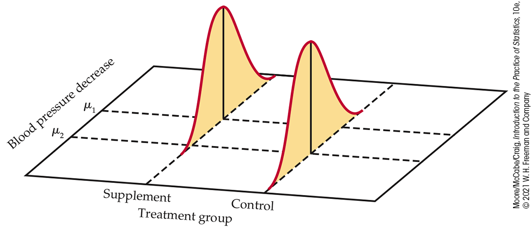
Figure 10.1 The statistical model for comparing responses to two treatments; the mean response varies with the treatment.
Statistical model for linear regression
In linear regression, the explanatory variable x is
quantitative and can have many different values. Imagine, for example,
giving different doses of the calcium supplement x to different
groups. We can think of the values of x as defining different
subpopulations, one for each possible value of x. Each subpopulation
consists of all individuals in the population having the same value of
x. If we gave an
The statistical model for simple linear regression assumes that for
each value of x (or subpopulation), the response variable
y is Normally distributed, with a mean that depends on
x. We use
-
The mean blood pressure decrease is different for the different
subpopulations of x. The means all lie on a straight line.
That is,
-
Individual blood pressure decreases y within each
subpopulation of x vary according to a Normal distribution.
This variation, measured by the standard deviation
The simple linear regression model is pictured in
Figure 10.2. The line describes how the mean response
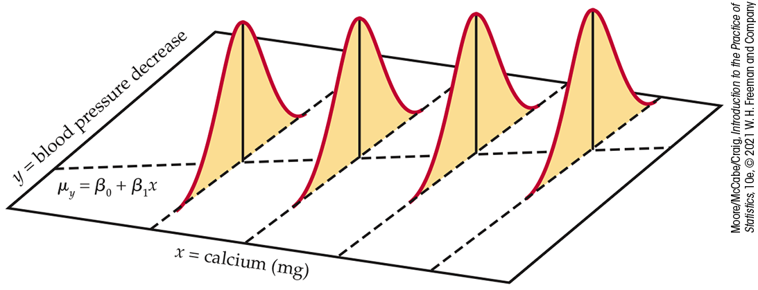
Figure 10.2 The statistical model for linear regression; the mean response is a straight-line function of the explanatory variable.
Preliminary data analysis and inference considerations
The data for a linear regression are the n observed (x, y) pairs. The model takes each x to be a known quantity, like the milligrams of the calcium supplement.1 The response y for a given x is assumed to be a Normal random variable. The linear regression model describes the mean and standard deviation of this random variable.
We use the following example to explain the fundamentals of simple linear regression. Because regression calculations in practice are done by statistical software, we rely on computer output for the arithmetic. In Section 10.2, we show formulas to do the work with a calculator or spreadsheet. These formulas are useful in understanding analysis of variance (Section 10.2) and multiple regression (Chapter 11).
Example 10.1 Relationship between BMI and physical activity.
![]()

Decrease in physical activity is considered to be a major contributor to the increase in prevalence of overweight and obesity in the general adult population. Because the prevalence of physical inactivity among college students is similar to that of the adult population, researchers have tried to understand college students’ physical activity perceptions and behaviors.
In several studies, researchers have looked at the relationship
between physical activity (PA) and body mass index (BMI).2
For this study, each participant wore a FitBit Flex™ for a week, and
the average number of steps taken per day (in thousands) was
recorded. Various body composition variables, including BMI in
kilograms per square meter,
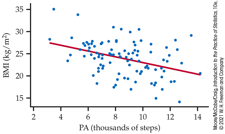
Figure 10.3 Scatterplot of body mass index (BMI) versus physical activity (PA) with the least-squares line, Example 10.1.
We start our analysis with a scatterplot of the data. Figure 10.3 is a plot of BMI versus physical activity for our sample of 100 participants. We use the names BMI and PA for the two quantitative variables. The least-squares regression line is included in the plot. There is a negative association between BMI and PA that appears approximately linear. There is also a considerable amount of scatter about this line.
Always start with a graphical display of the data.
![]() There is no point in fitting a linear model if the relationship is
not approximately linear.
A graphical display can also be used to assess the direction and
strength of the relationship and to identify outliers and influential
observations.
There is no point in fitting a linear model if the relationship is
not approximately linear.
A graphical display can also be used to assess the direction and
strength of the relationship and to identify outliers and influential
observations.
Before continuing our analysis, it is appropriate to consider the
extent to which the results can reasonably be generalized. In the
original study, undergraduate volunteers were obtained at a large
southeastern public university through
classroom announcements and campus flyers.
![]() The potential for bias should always be considered when obtaining
volunteers.
In this study, the volunteers were screened, and those with severe
health issues, as well as varsity athletes, were excluded. As a
result, the researchers considered the participants as an SRS from the
population of undergraduates at this university. However, they
acknowledged the risks of generalizing further, stating that similar
investigations at universities of different sizes and in other
climates of the United States are needed.
The potential for bias should always be considered when obtaining
volunteers.
In this study, the volunteers were screened, and those with severe
health issues, as well as varsity athletes, were excluded. As a
result, the researchers considered the participants as an SRS from the
population of undergraduates at this university. However, they
acknowledged the risks of generalizing further, stating that similar
investigations at universities of different sizes and in other
climates of the United States are needed.
Revisiting the simple linear regression model
In this example, subpopulations are defined by the explanatory variable x, physical activity. The considerable amount of scatter about the least-squares regression line suggests a large amount of variation of BMI for each value of x that is in each subpopulation. Why might this occur? Consider sampling women from your university, each averaging the same number of steps per day—say, 9000. Even though the average number of steps per day is the same, you would not expect all these women to have the same BMI. Variation in other factors, such as genetic makeup, lifestyle, and diet should all contribute to the variation of BMI.
The statistical model for linear regression assumes that these BMI
values are Normally distributed, with a mean
This was displayed in Figure 10.2 with the line and the four Normal curves. The line is the population regression line, which gives the average BMI for all values of x. The Normal curves provide a description of the variation of BMI about these means.
The following equation expresses this idea:
The FIT part of the model consists of the subpopulation means, given
by the expression
We use
Check-in
-
10.1 Understanding a linear regression model. Consider a linear regression model for the decrease in blood pressure (mmHg) over a four-week period with
-
What is the slope of the population regression line?
-
Explain clearly what this slope says about the change in the mean of y for a 100 mg increase in x.
-
What is the intercept of the population regression line?
-
Explain clearly what this intercept says about the mean decrease in blood pressure.
-
-
10.2 Understanding a linear regression model, continued. Refer to the previous Check-in question.
-
What is the subpopulation mean when the supplement is
-
What is the subpopulation distribution when the supplement is
-
Using the 68–95–99.7 rule (page 51), between what two values would approximately 95% of the observed responses y fall when
-
Before moving on to parameter estimation, there is one additional
issue that often deserves attention. The simple linear regression
model considers that the x-values are known exactly but, in
practice, they are often estimated. For example, in our study, the
physical activity level x is estimated using a FitBit Flex worn
over a one-week period.
![]() If there is error in measuring x, and it is large relative to the
spread of the x’s, more advanced inference methods using
errors-in-variables models are needed.
In this case, the
measurement
error
is expected to be relatively small. Subjects were instructed to
continue normal activities and to notify the researchers of any
deviations. Also, this estimate of physical activity represents an
average over seven days.
If there is error in measuring x, and it is large relative to the
spread of the x’s, more advanced inference methods using
errors-in-variables models are needed.
In this case, the
measurement
error
is expected to be relatively small. Subjects were instructed to
continue normal activities and to notify the researchers of any
deviations. Also, this estimate of physical activity represents an
average over seven days.
Estimating the regression parameters
The method of least squares presented in
Chapter 2 fits a line
to summarize a relationship between the observed values of an
explanatory variable and a response variable. Now we want to use the
least-squares regression line as a basis for inference about a
population from which our observations are a sample. In that setting,
the slope
estimate the slope
![]() This inference should only be done when the linear regression model
conditions are reasonably met.
Various checks are needed, and some judgment is required. Because
additional methods to check these conditions rely on first fitting the
model to the data, let’s briefly review the estimation methods of
Chapter 2.
This inference should only be done when the linear regression model
conditions are reasonably met.
Various checks are needed, and some judgment is required. Because
additional methods to check these conditions rely on first fitting the
model to the data, let’s briefly review the estimation methods of
Chapter 2.
Using the formulas from Chapter 2, the slope of the least-squares line is
and the intercept is
Here, r is the correlation between the observed values of
y and x,
Recall that the least-squares regression line always passes through
the point
The remaining parameter to be estimated is
Recall that the vertical deviations of the points in a scatterplot
from the fitted regression line are the residuals. We use
The residuals
To estimate
We average by dividing the sum by
We call s the regression standard error.
We now use statistical software to calculate the regression for predicting BMI from physical activity for Example 10.1. In entering the data, we chose the names PA for the explanatory variable and BMI for the response. It is good practice to use names, rather than just x and y, to remind yourself which variables the output describes.
Example 10.2 Statistical software output for BMI and physical activity.
![]()
Figure 10.4
gives the outputs from two commonly used statistical software
packages and Excel. Other software will give similar information.
The JMP output reports estimates of our three parameters as
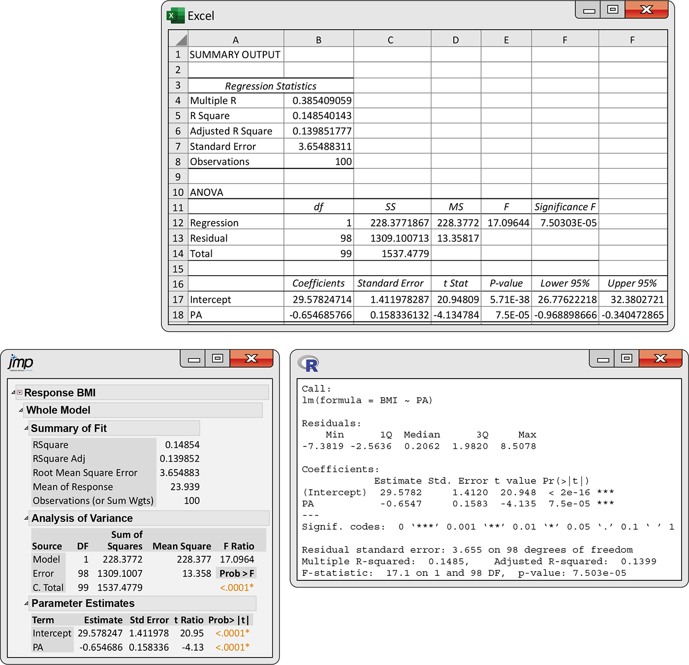
Figure 10.4 Regression outputs from Excel, JMP, and R, Example 10.2.
The least-squares regression line is the straight line that is plotted in Figure 10.3 (page 518). We would report it as
with an estimated model standard deviation of
Note that the number of digits provided varies with the software used,
and we have rounded the values to three decimal places. It is
important to avoid cluttering up your report of the results of a
statistical analysis with many digits that are not relevant.
![]() Software often reports many more digits than are meaningful or
useful.
Software often reports many more digits than are meaningful or
useful.
Computer outputs often give more information than we want or need. This is done to reduce user frustration when a software package does not print out the particular statistics wanted for an analysis. As you gain experience interpreting output, you learn to ignore the parts of the output that are not needed for the current analysis.
Example 10.3 Predicted values and residuals for BMI.
We can use the least-squares regression equation to find the predicted BMI corresponding to any value of PA. Suppose that a female college student averages 8000 steps per day. We predict that this person will have a BMI of
If her actual BMI is 25.655, then the residual would be
Because the means
![]() However, extreme caution must be taken when performing inference
for an x-value outside the range of the observed x’s, also known as
extrapolation, because there is no assurance that the same linear
relationship between
However, extreme caution must be taken when performing inference
for an x-value outside the range of the observed x’s, also known as
extrapolation, because there is no assurance that the same linear
relationship between
Check-in
-
10.3 More on BMI and physical activity. Refer to Examples 10.2 (page 522) and 10.3.
-
What is the predicted BMI for a woman who averages 9500 steps per day?
-
If an observed BMI at
-
Suppose that you wanted to use the estimated population regression line to examine the predicted BMI for a woman who averages 4000, 10,000, or 16,000 steps per day. Discuss the appropriateness of using the least-squares equation to predict BMI for each of these activity levels.
-
Checking conditions for regression inference
Now that we have fitted a line, we can further check the conditions
that the simple linear regression model imposes on this fit. These
checks are very important but often overlooked.
![]() There is no point in trying to do statistical inference if the data
do not, at least approximately, meet the conditions that are the
foundation for the inference.
Misleading or incorrect conclusions can result.
There is no point in trying to do statistical inference if the data
do not, at least approximately, meet the conditions that are the
foundation for the inference.
Misleading or incorrect conclusions can result.
These conditions concern the population, but we can observe only our sample. Thus, in doing inference, we act as if the sample is an SRS from the population. When the data are collected through some sort of random sampling, this condition is often easy to justify. In other settings, this condition requires more thought, and the justification is often debatable. For example, in Example 10.1 (page 518), the sample was a collection of volunteers, and the researchers argued that they could be considered an SRS from the population of college students at that university.
The remaining model conditions can be checked through a visual examination of the residuals. The first condition is that there is a linear relationship in the population, and the second is that the standard deviation of the responses about the population line is the same for all values of the explanatory variable. It is common to plot the residuals both against the case number (especially if this reflects the order in which the observations were collected) and against the explanatory variable. These residual plots are preferred to scatterplots of y versus x because they better magnify patterns. We often add a scatterplot smoother to these plots for further assistance in detecting patterns. The final condition is that the response varies Normally about the population regression line. That is, the model deviations vary Normally about 0.
Example 10.4 Checking the model conditions for BMI and physical activity.
![]()
Figure 10.5 is a plot of the residuals versus physical activity with a smooth-function fit. This smooth function suggests that the average residual is greater than 0 at both low and high physical activity levels. This could mean that a curved relationship between BMI and physical activity would better fit the data. It also could just be the result of chance variation. Notice that there is a large positive residual near each end of the physical activity range that is likely pulling up each end of the smoothed curve. Because the effect does not appear large, we attribute this pattern to chance variation. We do, however, investigate this further in Exercise 11.35 (page 593).
To check the assumption of a common standard deviation, we look at the spread of the residuals across the range of x. In Figure 10.5, the spread is roughly uniform across the range of PA, suggesting that this condition is reasonably met. There also do not appear to be any outliers or influential observations.
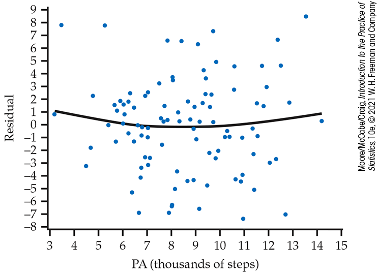
Figure 10.5 Plot of residuals versus physical activity (PA) with a smooth function, Example 10.4.
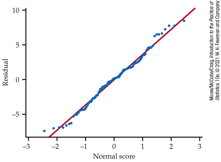
Figure 10.6 Normal quantile plot of the residuals, Example 10.4.
Figure 10.6 is a Normal quantile plot of the residuals. Because the plot looks reasonably straight, we are confident that the model deviations are approximately Normally distributed.
Note that the model does not require the distributions of y and
x to be Normal; only the distribution of the model deviations
is assumed Normal.
![]() It is a common mistake to assess the Normality of y when checking
model conditions.
Even though the examination of the x and y distributions
can be helpful in terms of identifying potential outliers and
influential observations, the focus should be on the residuals, which
account for the differing means, when checking Normality.
It is a common mistake to assess the Normality of y when checking
model conditions.
Even though the examination of the x and y distributions
can be helpful in terms of identifying potential outliers and
influential observations, the focus should be on the residuals, which
account for the differing means, when checking Normality.
In settings where the choices of x are controlled—for example, assigning subjects different milligrams of calcium supplement—we consider the subjects to be an SRS from the population and that they are randomly assigned to the different choices of x. In other words, the y’s for each value of x are an SRS from its subpopulation.
Provided our check of conditions gives no reason to question the use of the simple linear regression model, we can comfortably proceed to inference about parameters, or functions of parameters, such as
-
The slope
-
The mean response
- An individual future response y for a given value of x.
If these condition checks raise doubts, it is best to consult an expert, as a more sophisticated regression model is likely needed. There is, however, one relatively simple remedy that may be worth investigation: transforming variables. An example using this remedy is provided at the end of this section.
Confidence intervals and significance tests
![]()
Chapter 7 presented confidence intervals and significance tests for means and differences in means. In each case, inference rested on the standard errors of estimates and on t distributions. Inference in simple linear regression is similar in principle. For example, the confidence intervals have the form
where
As a consequence of the model assumptions about the deviations
Because we do not know
Formulas for confidence intervals and significance tests for the
intercept
The test of
This equation says that the mean of y does not vary with
x. In other words, all the y’s come from a single
population with mean
Example 10.5 Statistical software output, continued.
The computer outputs in
Figure 10.4 (page 522) for the physical activity study contain the information needed
for inference about the regression slope and intercept. Let’s look
at the JMP output. The column labeled “Std Error” gives the standard
errors of the estimates. The value of
The t statistic and P-value for the test of
The P-value is given as
We have found a statistically significant linear relationship between physical activity and BMI. The estimated slope is more than 4 standard deviations away from zero. Because this is highly unlikely to happen if the true slope is zero, we have strong evidence for our claim.
Note, however, that this is not the same as concluding that we have
found a strong linear relationship between the response and
explanatory variables in this example. We saw in
Figure 10.3 that there is a
lot of scatter about the regression line.
![]() A very small P-value for the significance test for a zero slope
does not necessarily imply that we have found a strong
relationship.
A very small P-value for the significance test for a zero slope
does not necessarily imply that we have found a strong
relationship.
A confidence interval provides additional information about the linear relationship. For most statistical software, these intervals are optional output and must be requested. We can also construct them by hand from the default output.
Example 10.6 Confidence interval for the slope.
A confidence interval for
To compute the 95% confidence interval for
The interval is
We mentioned earlier that the intercept in this example is not of
practical interest. It estimates average BMI when the activity level
is 0, a value that isn’t realistic. For this reason, we do not compute
a confidence interval for
Check-in
-
10.4 Significance test for the population slope. Test the null hypothesis that the slope is zero versus the two-sided alternative in each of the following settings using the
-
-
10.5 95% confidence interval for the slope. For each of the settings in the previous Check-in question, find the 95% confidence interval for the slope and explain what the interval tells you.
Confidence intervals for mean response
Besides performing inference about the slope (and sometimes the intercept) in a linear regression, we may want to use the estimated regression line to make predictions about the response y at certain values of x. We may be interested in the mean response for different subpopulations or in the response of future observations at different values of x. In either case, we would want an estimate and associated margin of error.
For any specific value of x, say
To estimate this mean from the sample, we substitute the estimates
A confidence interval for
Many computer programs calculate confidence intervals for the mean
response corresponding to each of the x-values in the data.
Some can calculate an interval for any value
Example 10.7 Confidence intervals for the mean response.
![]()
Figure 10.7
shows the upper and lower confidence limits on a graph with the data
and the least-squares line. The 95% confidence limits appear as
dashed curves. For any
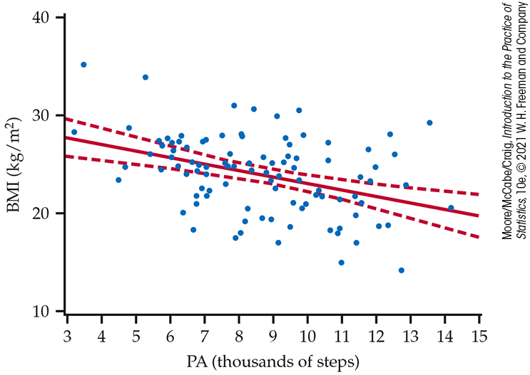
Figure 10.7 The 95% confidence limits (dashed curves) for the mean response for the physical activity study, Example 10.7.
Some software will do these calculations directly if you input a value for the explanatory variable. Other software will calculate the intervals for each value of x in the data set. Creating a new data set with an additional observation with x equal to the value of interest and y missing will often work.
Example 10.8 Confidence interval for an average of 9000 steps per day.
Let’s find the confidence interval for the average BMI at
Software tells us that the 95% confidence interval for the mean
response is 23.0 to 24.4
If we sampled many women who averaged 9000 steps per day, we would
expect their average BMI to be between 23.0 and 24.4
![]() These confidence intervals do not tell us what BMI to expect for a
single observation at a particular average steps per day.
We need a different kind of interval, a prediction interval, for this
purpose.
These confidence intervals do not tell us what BMI to expect for a
single observation at a particular average steps per day.
We need a different kind of interval, a prediction interval, for this
purpose.
Prediction intervals
![]()
In the last example, we predicted the average BMI for
This is the same as the expression for
This means our best guess for the BMI of this woman averaging 9000
steps per day is what we obtained using the regression equation,
Consider doing the following many times:
-
Draw a sample of n observations
-
Calculate the 95% prediction interval for y when
Then, 95% of the prediction intervals will contain the value of y for the additional observation. In other words, the probability that this method produces an interval that contains the value of a future observation is 0.95.
The form of the prediction interval is very similar to that of the
confidence interval for the mean response. The difference is that the
standard error
Again, we use a graph to illustrate the results.
Example 10.9 Prediction intervals for BMI.
![]()
Figure 10.8 shows the upper and lower prediction limits, along with the data and the least-squares line. The 95% prediction limits are indicated by the dashed curves. Compare this figure with Figure 10.7, which shows the 95% confidence limits drawn to the same scale. The upper and lower limits of the prediction intervals are much farther away from the least-squares line than are the confidence limits. This results in most, but not all, of the observations in Figure 10.8 lying within the prediction bands.
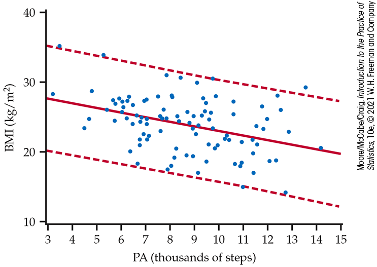
Figure 10.8 The 95% prediction limits (dashed curves) for individual responses for the physical activity study, Example 10.9. Compare with Figure 10.7. The limits are wider because the margins of error incorporate the variability about the subpopulation means.
The comparison of Figures 10.7 and 10.8 reminds us that the interval for a single future observation must be larger than an interval for the mean of its subpopulation.
Example 10.10 Prediction interval for 9000 steps per day.
Let’s find the prediction interval for a future observation of BMI
for a college-aged woman who averages 9000 steps per day. The
predicted value is the same as the estimate of the average BMI that
we calculated in
Example 10.8 (that is,
![]() Although a larger sample would better estimate the population
regression line, it would not reduce the degree of scatter about the
line.
This means that prediction intervals for BMI, given activity level,
will always be wide. This example clearly demonstrates that a
very small P-value for the significance test for a zero slope
does not necessarily imply that we have found a strong predictive
relationship.
Although a larger sample would better estimate the population
regression line, it would not reduce the degree of scatter about the
line.
This means that prediction intervals for BMI, given activity level,
will always be wide. This example clearly demonstrates that a
very small P-value for the significance test for a zero slope
does not necessarily imply that we have found a strong predictive
relationship.
Check-in
-
10.6 Margin of error for the predicted mean. Refer to Figure 10.7 (page 529) and Example 10.8 (page 529). What is the 95% margin of error of
-
10.7 Margin of error for a predicted response. Refer to Example 10.10. What is the 95% margin of error of
Transforming variables
We started our analysis of Example 10.1 with a scatterplot to check whether the relationship between BMI and physical activity could be summarized with a straight line. We followed the least-squares fit with a residual plot (Figure 10.5) and a Normal quantile plot (Figure 10.6) to check that Normality, constant standard deviation, and linearity were approximately met. A check of model conditions should always be done prior to inference.
When there is a violation, it is best to consult an expert. However, there are times when a transformation of one or both variables will remedy the situation. In Chapter 2, we discussed the use of the log transformation to describe a curved relationship between x and y. Here is an example where the log transformation has a greater impact on other model assumptions.
Example 10.11 The relationship between income and education for entrepreneurs.
![]()
Numerous studies have shown that better-educated employees have higher incomes. Is this also true for entrepreneurs? Do more years of formal education translate into higher incomes? One study explored this question using the National Longitudinal Survey of Youth (NLSY), which followed a large group of individuals aged 14 to 22 for roughly 10 years.3 We consider a random sample of 100 entrepreneurs.
The researchers defined entrepreneurs to be those who were self-employed or who were the owner/director of an incorporated business. For each of these individuals, they recorded the education level and income. The education level was defined as the years of schooling completed prior to starting the business. The income level was the average annual total earnings since starting the business.
Figure 10.9 is a scatterplot of income versus education for our sample of 100 entrepreneurs, along with a smoothed curve. We use the variable names Inc and Educ.
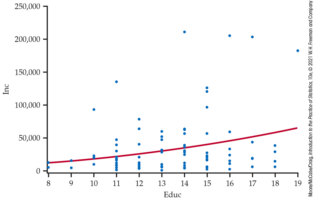
Figure 10.9 Scatterplot, with smoothed curve, of average annual income versus years of education for a sample of 100 entrepreneurs, Example 10.11.
The smoothed curve looks roughly linear, but the distributions of income subpopulations are skewed to the right. At each education level, there are many small incomes and just a few very large incomes. It also looks like the smoothed curve is being pulled toward those very large incomes, suggesting that those observations could be influential.
A common remedy for a skewed variable is to consider transforming it prior to fitting the model. Here, the researchers considered the natural logarithm of income (LogInc).
Example 10.12 Is this linear regression model reasonable?
![]()
Figure 10.10 is a scatterplot of these transformed data with the least-squares line and smoothed curve. Notice that the smoothed curve is practically the same as the least-squares line. More importantly, the observations are now more equally dispersed above and below the line, and those very large incomes don’t look unusual anymore.
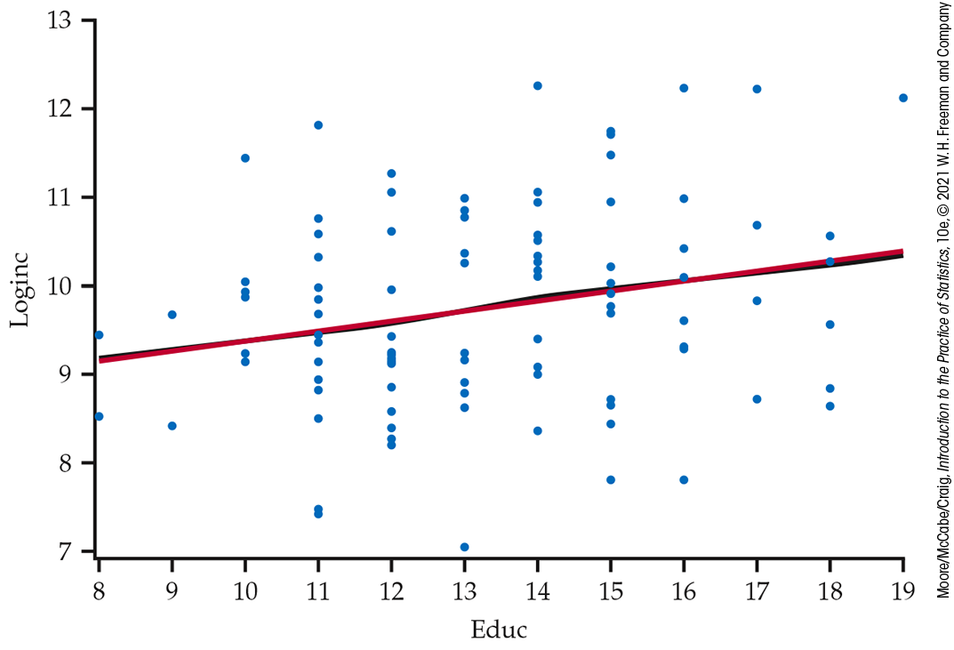
Figure 10.10 Scatterplot, with smoothed curve (black) and regression line (red), of log average annual income versus years of education for a sample of 100 entrepreneurs. The smoothed curve is almost the same as the least-squares regression line, Example 10.12.
A complete check of the residuals is still needed (see
Exercise 10.13), but it
appears that transforming y results in a data set that
satisfies the linear regression model. Not only is the relationship
more linear but the distribution of the observations about the
regression line is more Normal.
![]() This is not always the end result of a transformation. In other
cases, transforming a variable may help linearity and harm the
Normality and constant variance assumptions. Always check the
residuals before proceeding with inference.
This is not always the end result of a transformation. In other
cases, transforming a variable may help linearity and harm the
Normality and constant variance assumptions. Always check the
residuals before proceeding with inference.
Example 10.13 The accumlation of bone mass in young women.
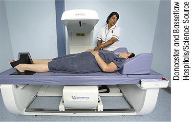
As we age, our bones become weaker and are more likely to break. Osteoporosis (or weak bones) is the major cause of bone fractures in older women. Various researchers have studied this problem by looking at how and when bone mass is accumulated by young women. They’ve determined that up to 90% of a person’s peak bone mass is acquired by age 18 in girls.4 This makes youth the best time to invest in stronger bones.
Figure 10.11
displays data for a measure of bone strength called “total body bone
mineral density” (TBBMD) and age for a sample of 256 young
women.5
TBBMD is measured in grams per square centimeter
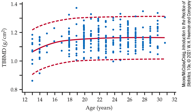
Figure 10.11 Plot of total body bone mineral density versus age, Example 10.13.
The fitted nonlinear equation is
In this equation,
The long-range goals of the researchers who conducted this study include developing intervention programs (such as exercise and increasing calcium intake) for young women to increase their TBBMD.
Section 10.1 SUMMARY
-
The simple linear regression model says that the means of the response variable y fall on a line when plotted against x, with the observed y’s varying Normally about these means. For n observations, this model can be written
for
-
The parameters of the model are the intercept
where the
-
Prior to inference, always check the model conditions by examinng the residuals for Normality, constant variance, and any other remaining patterns in the data. Plots of the residuals both against the case number and against the explanatory variable are commonly part of this examination.
-
A level C confidence interval for the slope
where
-
The test of the hypothesis
and the
-
The estimated mean response for the subpopulation corresponding to the value
-
The estimated value of the response variable for a future observation from the subpopulation corresponding to the value
-
A level C confidence interval for the mean response
where
-
A level C prediction interval for a future response y when
where
-
The standard error for the prediction interval is larger than the confidence interval because it also includes the variability of the future observation around its subpopulation mean.
-
Sometimes, a transformation of one or both of the variables can make their relationship linear. However, these transformations can harm other conditions, like Normality and constant variance, so it is important to examine the residuals.
Section 10.1 EXERCISES
-
10.1 What’s wrong? For each of the following statements, explain what is wrong and why.
-
The parameters of the simple linear regression model are
-
To test
-
For a particular value of the explanatory variable x, the confidence interval for the mean response will be wider than the prediction interval for a future observation.
-
-
10.2 What’s wrong? For each of the following statements, explain what is wrong and why.
-
The slope describes the change in x for a change in y.
-
The population regression line is
-
A 95% confidence interval for the mean response is the same width, regardless of x.
-
-
10.3 U.S. versus overseas stock returns. Returns on common stocks in the United States and overseas appear to be growing more closely correlated as economies become more interdependent. Suppose that the following population regression line connects the total annual returns (in percent) on two indexes of stock prices:
-
What is
-
What is
-
We know that overseas returns will vary in years when U.S. returns do not vary. Write the regression model based on the population regression line given above. What part of this model allows overseas returns to vary when U.S. returns remain the same?
-
-
10.4 Predicting BMI. In Example 10.2, Subject 13 averaged 9114 steps and has a BMI of 29.9. Using the least-squares regression equation in Example 10.3, find the predicted BMI and the residual for this individual.
-
 10.5 Importance of Normal model deviations?
A general form of the central limit theorem tells us that the
sampling distributions of
10.5 Importance of Normal model deviations?
A general form of the central limit theorem tells us that the
sampling distributions of
-
10.6 College debt versus adjusted in-state costs. Kiplinger’s “Best Values in Public Colleges” provides a ranking of U.S. public colleges based on a combination of various measures of academics and affordability.6 Let’s focus on the relationship between the average debt in dollars at graduation (AveDebt) and the in-state cost per year after need-based aid (InCostAid). A scatterplot that includes the least-squares regression line is shown in Figure 10.12 for a random sample of 27 colleges from the 2019 report.

-
Does a linear relationship between InCostAid and AveDebt seem reasonable? Explain your answer.
-
Are there any unusual cases in this sample? If yes, state which ones they are and how they may be affecting the least-squares fit.
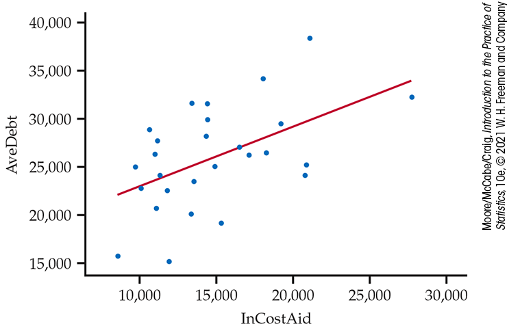
Figure 10.12 Scatterplot with least-squares regression line, Exercise 10.6.
-
-
10.7 Can we consider this an SRS? Refer to the previous exercise. The report states that Kiplinger’s rankings focus on traditional four-year public colleges with broad-based curricula and on-campus housing. Each year, Kiplinger starts with more than 500 schools and then narrows down the list to roughly the top 150, based on academic quality. The data set in the previous exercise is an SRS from Kiplinger’s published list of 174 schools. In terms of investigating the relationship between the average debt and the in-state cost after adjusting for need-based aid, is it reasonable to consider this to be an SRS from the population of more than 500 schools? Write a short paragraph explaining your answer.
-
10.8 Predicting college debt. Refer to Exercise 10.6. Colorado School of Mines has a much larger in-state cost than the other schools in the sample. Figure 10.13 contains JMP output for the simple linear regression of AveDebt on InCostAid with this case removed.
State the least-squares regression line.
-
Construct a 95% confidence interval for the slope. What does this interval tell you about the change in average debt for a $1000 increase in the in-state cost?
-
Indiana University Bloomington is one school in this sample. It has an in-state cost of $10,632 and average debt of $28,792. What is the residual?
-
Penn State University is reported to have an adjusted in-state cost of $25,235. Discuss the appropriateness of using this revised data set to predict the average debt for this university.
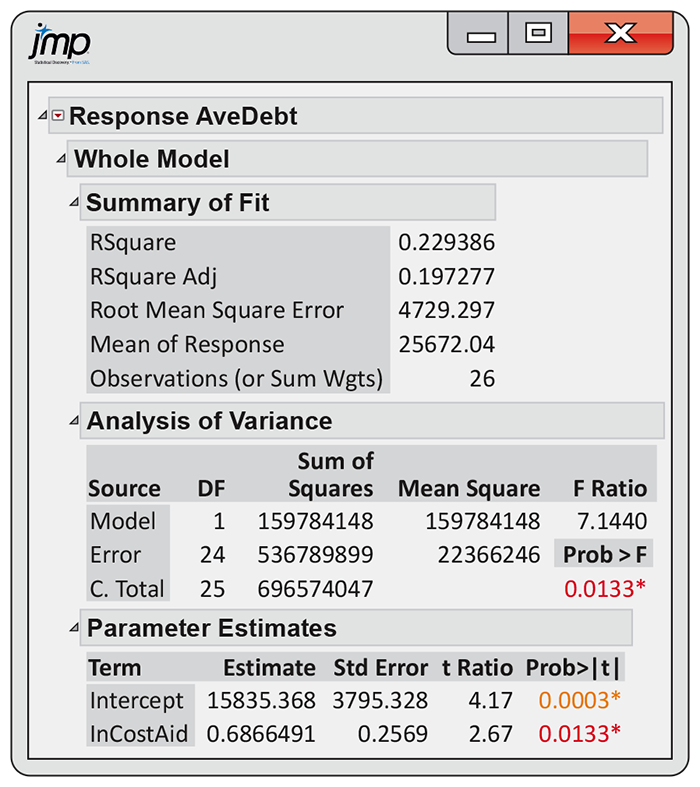
Figure 10.13 JMP output for the simple linear regression, Exercise 10.8.
-
10.9 More on predicting college debt. Refer to the previous exercise. James Madison University has an in-state cost of $15,659, and University of Wisconsin–Madison has an in-state cost of $11,507.
-
Using your answer to part (a) of the previous exercise, what is the predicted average debt for a student at James Madison University?
-
What is the predicted average debt for a student at University of Wisconsin–Madison?
-
Without doing any calculations, would the 95% margin of error for the predicted average debt be larger for James Madison University or the University of Wisconsin–Madison? Explain your answer.
-
-
10.10 Impact of an unusual observation. Refer to Exercise 10.6 (page 536). Colorado School of Mines was removed from this analysis because it was considered an influential observation. Is that the case? Let’s investigate its impact on the fit.
-
Refit the model using the entire sample of 27 schools. Create a table that summarizes the model estimates with and without this case.
-
Describe the impact this observation has on the fit of the linear regression model.
-
If you were writing a report for publication, would you include the fit with or without this case? Explain your answer.
-
-
10.11 Predicting college debt: Other measures. Refer to Exercise 10.6. Let’s look at AveDebt and its relationship with the other explanatory variables in the data set. In addition to the in-state cost after aid (InCostAid), there is the admittance rate (Admit), the four-year graduation rate (Grad4Rate), and the in-state cost before aid (InCost).
-
Generate scatterplots of each explanatory variable and AveDebt. Do all these relationships look linear? Describe what you see. Does Colorado School of Mines still look influential? Do any new cases raise alarms?
-
Fit each of the explanatory variables separately and create a table that lists the explanatory variable, the estimated model standard deviation s, and the P-value for the test of a linear association. For each analysis, make sure to specify whether you remove any observations or not.
-
Which variable do you think is the best single explanatory variable of average debt? Explain your answer.
-
-
10.12 Complete check of the residuals. In Example 10.11 (page 532), we checked model assumptions using a scatterplot (Figure 10.9). Let’s consider assessing the model assumptions using the residuals.

-
Fit the (Educ, Inc) data using least-squares regression and obtain the residuals. Write down the least-squares regression line.
-
Generate a plot of the residuals versus Educ and comment on the pattern. Does a linear fit appear reasonable? Does there appear to be constant variance? Are there any unusual observations? Explain your answers.
-
Construct a histogram or a Normal quantile plot of the residuals. Do the residuals appear Normal? Explain your answer.
-
Analysis of the residuals is typically done because patterns in the residuals are easier to see. Do you think the plots in parts (b)and (c) magnify the violations of assumptions better than the scatterplot in Figure 10.9? Write a short paragraph comparing the scatterplot with the residual plots.
-
-
10.13 Complete check of the residuals, continued. Refer to the previous exercise. In Example 10.12 (page 533), we checked model assumptions using a scatterplot (Figure 10.10) after log transforming the response variable.
-
Repeat parts (a) through (c) of the previous exercise using LogInc and Educ.
-
Do you think we can comfortably perform inference using the log transformed y? Explain your answer.
-
-
10.14 Are the two fuel-efficiency measurements similar? Refer to Exercise 7.18 (page 407). In addition to the computer calculating miles per gallon (mpg), the driver also measured mpg by dividing the miles driven by the number of gallons at fill-up. The driver wants to determine if these calculations are similar.

Fill-up 1 2 3 4 5 6 7 8 9 10 Computer 41.5 50.7 36.6 37.3 34.2 45.0 48.0 43.2 47.7 42.2 Driver 36.5 44.2 37.2 35.6 30.5 40.5 40.0 41.0 42.8 39.2 Fill-up 11 12 13 14 15 16 17 18 19 20 Computer 43.2 44.6 48.4 46.4 46.8 39.2 37.3 43.5 44.3 43.3 Driver 38.8 44.5 45.4 45.3 45.7 34.2 35.2 39.8 44.9 47.5 -
Consider the driver’s mpg calculations as the explanatory variable. Plot the data and describe the relationship. Are there any outliers or unusual values? Does a linear relationship seem reasonable?
-
Run the simple linear regression and state the least-squares regression line.
-
Summarize the results. Does it appear that the computer and driver calculations are the same? Explain your answer.
-
-
10.15 Is the number of tornadoes increasing? The Storm Prediction Center of the National Oceanic and Atmospheric Administration maintains a database of tornadoes, floods, and other weather phenomena. TABLE 10.1 summarizes the annual number of tornadoes in the United States between 1953 and 2019.7 (Note: These are time series data with weak autocorrelation, so simple linear regression is reasonable here.)

Table 10.1 Annual number of tornadoes in the United States between 1953 and 2019
Year Number of tornadoes Year Number of tornadoes Year Number of tornadoes Year Number of tornadoes 1953 422 1970 654 1987 658 2004 1813 1954 550 1971 888 1988 700 2005 1262 1955 591 1972 740 1989 859 2006 1106 1956 504 1973 1104 1990 1140 2007 1100 1957 857 1974 951 1991 1133 2008 1692 1958 564 1975 918 1992 1302 2009 1146 1959 602 1976 837 1993 1174 2010 1282 1960 616 1977 854 1994 1085 2011 1691 1961 698 1978 789 1995 1236 2012 938 1962 656 1979 859 1996 1172 2013 906 1963 462 1980 866 1997 1149 2014 886 1964 706 1981 782 1998 1428 2015 1177 1965 900 1982 1049 1999 1342 2016 976 1966 585 1983 930 2000 1073 2017 1429 1967 927 1984 912 2001 1212 2018 1126 1968 661 1985 687 2002 934 2019 1276 1969 607 1986 765 2003 1385 -
Make a plot of the total number of tornadoes by year. Does a linear trend over years appear reasonable? Are there any outliers or unusual patterns? Explain your answer.
-
Run the simple linear regression and report the least-squares regression line.
-
A friend of yours thinks you made a mistake fitting the model because
-
Obtain the residuals and plot them versus year. Are there any unusual patterns or cases that you did not discuss in part (a)? If so, comment on them.
-
Are the residuals approximately Normal? Justify your answer.
-
Based on the these residual checks, are you confident proceeding with inference? Explain your answer.
-
-
10.16 Annual increase? Refer to the previous exercise. Let’s proceed with inference regardless of your confidence level.
-
Do these data support a linear trend in the number of tornadoes? Justify your answer.
-
Construct a 95% confidence interval for the average annual increase in the number of tornadoes. Explain how this interval can be used to justify your response in part (a).
-
What is the predicted number of tornadoes in 2020?
-
Provide an interval that should contain the actual count 95% of the time.
-
-
10.17 Computer memory. The capacity of memory commonly sold at retail has increased rapidly over time.8

-
Make a scatterplot of the data. The growth is much faster than linear.
-
Compute the logarithm of capacity and plot it against year. Are these points closer to a straight line?
-
Fit the simple linear regression model with logarithm of capacity as the response and year as the explanatory variable. Give a 90% confidence interval for the slope of the population regression line.
-
Write a brief summary describing the change in memory capacity over time using the confidence interval from part (c).
-
-
10.18 Alternative tornado model. Refer to
Exercise 10.15. Most
of the largest positive and negative deviations occur later in
time. This suggests that there may not be constant variance.
Because the response variable is a count, one can argue the
variance is not constant (e.g., see the Poisson distribution,
page 315).
-
Take the natural logarithm of the count and refit the model using this transformed response variable. Report the least-squares regression line.
-
Check the residuals of this model. Does the linear regression model fit these data? Explain your answer.
-
When the response y is on the log scale, the slope approximates the percent change in y for a unit increase in x. Construct an approximate 95% confidence interval for the annual percent change.
-
Does this model also support the hypothesis that tornadoes have increased over time? Explain your answer.
-
Construct a prediction interval for the predicted number of tornadoes in 2020 and compare it with the interval from part (d) of Exercise 10.19. (Note: An approximate interval can be constructed by first obtaining a prediction interval for
-
Which of the two models (and thus prediction) do you prefer? Explain your answer.
-