10.2 More Detail about Simple Linear Regression
In this section, we expand on three topics related to simple linear regression. The first is analysis of variance for regression. If you plan to read Chapter 11 on multiple regression or Chapters 12 and 13 on comparing several means, this information is helpful preparation. The second topic concerns the computations for regression inference. Even though we recommend using software for analysis, knowing the formulas provides some additional insights. To conclude, we discuss inference for correlation and its close connection to inference about the slope.
Analysis of variance for regression
The usual computer output for regression includes an additional block of calculations that is labeled “ANOVA” or “Analysis of Variance.” Analysis of variance, often abbreviated ANOVA, is the term for statistical analyses that break down the variation in the data into separate pieces that correspond to different sources of variation. It is closely related to the conceptual
framework we discussed earlier (page 519).
The total variation in the response y is expressed by the
deviations
-
As the explanatory variable x changes, the mean response changes with it along the regression line. For example, in Figure 10.3 (page 518), students averaging 10,000 steps generally have lower BMIs than those averaging 6000 steps. The fitted value
-
Individual observations vary Normally about their subpopulation mean. This variation is represented by the residuals
We can express the deviation of any y observation from the mean of the y’s as the sum of these two deviations. Specifically,
In terms of deviations, this equation expresses the idea that
Several times we have measured variation by taking an average of squared deviations. If we square each of the preceding three deviations and then sum over all n observations, it can be shown that the sums of squares add:
We rewrite this equation as
where
The SS in each abbreviation stands for sum of squares, and the T, M, and E stand for total, model, and error, respectively. (“Error” here stands for deviations from the line, which might better be called “residual” or “unexplained variation.”) The total variation, as expressed by SST, is the sum of the variation due to the straight-line model (SSM) and the variation due to deviations from this model (SSE). This partitioning of the variation in the data between two sources is the heart of analysis of variance.
The variation along the line, labeled SSM, is the variation among the
predicted responses
If
The numerator in this expression is SST. The denominator is the total degrees of freedom, or simply DFT.
Just as the total sum of squares SST is the sum of SSM and SSE, we partition the total degrees of freedom DFT as the sum of DFM and DFE, the degrees of freedom for the model and for the error:
The model has one explanatory variable x, so the degrees of
freedom for this source are
For each source, the ratio of the sum of squares to the degrees of freedom is called the mean square, or simply MS. The general formula for a mean square is
Each mean square is a type of average squared deviation. Mean square
total (MST) is just
It is our estimate of
In
Section 2.4
(page 107) we
noted that
Because SST is the total variation in y, and SSM is the
variation due to the regression of y on x, this equation
is the precise statement of the fact that
The ANOVA F test
The null hypothesis
When
The F distributions are a family of distributions with two parameters: the degrees of freedom of the mean square in the numerator and denominator of the F statistic. The F distributions are another of R. A. Fisher’s contributions to statistics and are called F in his honor. Fisher introduced F statistics for comparing several means. We meet these useful statistics in Chapters 12 and 13.
The numerator degrees of freedom are always mentioned first. Interchanging the degrees of freedom changes the distribution, so the order is important. Our brief notation will be F( j, k) for the F distribution with j degrees of freedom in the numerator and k in the denominator. The F distributions are not symmetric but are right-skewed. The density curve in Figure 10.14 illustrates the shape. Because mean squares cannot be negative, the F statistic takes only positive values, and the F distribution has no probability to the left of 0. The peak of the F density curve is near 1.
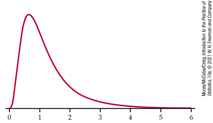
Figure 10.14 The density for the F(9, 10) distribution. The F distributions are skewed to the right.
Tables of F critical values are available for use when software
does not give the P-value or you cannot use a software
function, such as F.DIST.RT in Excel or pf in R. However, tables of
F critical values are awkward because
a separate table is needed for every pair of degrees of freedom.
Table E
in the back of the book contains the F critical values for
probabilities
The F statistic tests the same null hypothesis as the
t statistic for
The ANOVA calculations are displayed in an analysis of variance table, often abbreviated ANOVA table. Here is the format of the table for simple linear regression:
| Source | Degrees of freedom | Sum of squares | Mean square | F |
|---|---|---|---|---|
| Model | 1 |
|
SSM/DFM | MSM/MSE |
| Error |
|
|
SSE/DFE | |
| Total |
|
|
SST/DFT |
Example 10.14 Interpreting software output for BMI and physical activity.
![]()
The output generated by Minitab for the physical activity study in
Example 10.2
is given in
Figure 10.15. Note that Minitab uses the label “Regression” in place of
“Model.” Other software packages may use slightly different labels.
The F statistic is 17.10; the P-value is given as
0.000, which means
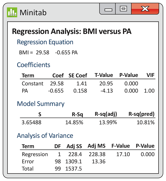
Figure 10.15 Minitab output for the physical activity study, Example 10.14.
Now look at the output for the regression coefficients. The
t statistic for PA is given as
![]() Strong evidence against the null hypothesis that there is no
relationship does not imply that a large percentage of the total
variability is explained by the model.
Strong evidence against the null hypothesis that there is no
relationship does not imply that a large percentage of the total
variability is explained by the model.
Check-in
-
10.8 Reading linear regression outputs. Figure 10.4 (page 522) shows the regression output from two software packages and Excel. Create a table that lists the labels each output uses in its ANOVA table, the F statistic, its P-value, and
-
10.9 Reading the ANOVA table. For the physical activity study, the regression standard error
Calculations for regression inference
We recommend using statistical software for regression calculations. With time and care, however, the work is feasible with a calculator or spreadsheet. We will use the following example to illustrate how to perform inference for regression analysis using a calculator.
Example 10.15 Umbilical cord diameter and gestational age.
![]()
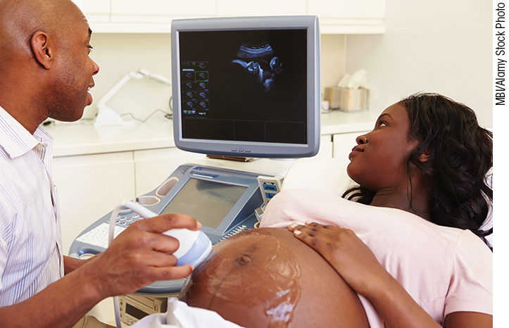
Knowing the gestational age (GA) of a fetus is important for biochemical screening tests and planning for successful delivery. Typically, GA is calculated as the number of days since the start of the woman’s last menstrual period (LMP). However, for women with irregular periods, GA is difficult to compute, and ultrasound imaging is often used. In the search for helpful ultrasound measurements, a group of Nigerian researchers looked at the relationship between umbilical cord diameter (mm) and gestational age based on LMP (weeks).9 Here is a small subset of the data:
| Umbilical cord diameter (x) | 2 | 6 | 9 | 14 | 21 | 23 |
| Gestational age (y) | 16 | 18 | 26 | 33 | 28 | 39 |
The data and the least-squares regression line are plotted in Figure 10.16. The strong straight-line pattern suggests that we can use linear regression to model the relationship between diameter and gestational age.
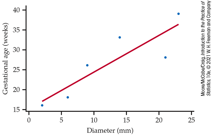
Figure 10.16 Scatterplot and least-squares regression line, Example 10.15.
We begin our regression calculations by fitting the least-squares
line. Fitting the line gives estimates
![]() Roundoff errors that accumulate during these calculations can ruin
the final results. Be sure to carry many significant digits and
check your work carefully.
For our work here, we will carry things to the fifth decimal place.
Roundoff errors that accumulate during these calculations can ruin
the final results. Be sure to carry many significant digits and
check your work carefully.
For our work here, we will carry things to the fifth decimal place.
Preliminary calculations
Because the scatterplot (Figure 10.16) suggests a straight-line pattern, we begin by fitting the least-squares line.
Example 10.16 Summary statistics for gestational age study.
![]()
We start by making a table with the mean and standard deviation for each of the variables, the correlation, and the sample size. These calculations should be familiar from Chapters 1 and 2. Here is the summary:
| Variable | Mean | Standard deviation | Correlation | Sample size |
|---|---|---|---|---|
| Diameter |
|
|
|
|
| Gestational age |
|
|
These quantities are the building blocks for our calculations.
We will need one additional quantity for the eventual standard
error calculations. It is the expression
Example 10.17 Computing the least-squares regression line.
Using the summary statistics provided in Example 10.16 and the formulas on pages 520–521, the slope of the least-squares line is
The intercept is
The equation of the least-squares regression line is therefore
This is the line shown in Figure 10.16.
Now that we have estimates of the first two parameters,
Example 10.18 Computing the predicted values and residuals.
![]()
The first observation is a diameter of
and the residual is
The residuals for the other diameters are calculated in the same
way. They are
Example 10.19
Computing
s 2
The estimate of
So the estimate of the standard deviation about the line is
Check-in
-
10.10 Computing the residuals. In Example 10.18, we computed the residual for the first observation and reported the residuals for the other five observations. Run through the calculations for the second and third observations to verify these values.

-
10.11 More on the model fitting check. In Example 10.18, we verified our calculations by checking that the residuals sum to zero. If they do not sum to zero, we either made an error in calculating the residuals or in calculating
Calculate the residuals under
Inference for slope and intercept
Confidence intervals and significance tests for the slope
Similarly, the standard deviation of
To estimate these standard deviations, we need only replace
The plot of the regression line with the data in Figure 10.16 shows a very strong relationship, but our sample size is small. We assess the situation with a significance test for the slope.
Example 10.20 Testing the slope.
First we find the standard error of the estimated slope:
To test
we calculate the t statistic:
Using
Table D
with
Two things are important to note about this example.
![]() First,
it is important to remember that we need to have a very large
effect if we expect to detect a slope different from zero with a
small sample size.
The estimated slope is more than 3.5 standard deviations away from
zero, but we are not much below the 0.05 standard for statistical
significance. Second, because we expect gestational age to increase
with increasing diameter, a one-sided significance test would be
justified in this setting.
First,
it is important to remember that we need to have a very large
effect if we expect to detect a slope different from zero with a
small sample size.
The estimated slope is more than 3.5 standard deviations away from
zero, but we are not much below the 0.05 standard for statistical
significance. Second, because we expect gestational age to increase
with increasing diameter, a one-sided significance test would be
justified in this setting.
The significance test tells us that the data provide sufficient
information to conclude that gestational age and umbilical cord
diameter are linearly related. We use the estimate
Example 10.21 Computing a 95% confidence interval for the slope.
Let’s find a 95% confidence interval for the slope
The interval is (0.220, 1.617). For each additional millimeter in diameter, the gestational age of the fetus is expected to be 0.220 to 1.617 weeks older.
In this example, the intercept
Confidence intervals for the mean response and prediction intervals for a future observation
When we substitute a particular value
-
We have estimated the mean response
-
We have predicted a future value of the response y.
The margins of error for these two uses are often quite different. Recall that prediction intervals for an individual response are wider than confidence intervals for estimating a mean response. We now proceed with the details of these calculations. Once again, standard errors are the essential quantities. And once again, these standard errors are multiples of s, our basic measure of the variability of the responses about the fitted line.
Note that the only difference between the formulas for these two standard errors is the extra 1 under the square root sign in the standard error for prediction. This standard error is larger due to the additional variation of individual responses about the mean response. This additional variation remains regardless of the sample size n and is the reason that prediction intervals are wider than the confidence intervals for the mean response.
For the gestational age example, we can think about the average gestational age for a particular subpopulation, defined by the umbilical cord diameter. The confidence interval would provide an interval estimate of this subpopulation mean. On the other hand, we might want to predict the gestational age for a new fetus. A prediction interval attempts to capture this new observation.
Example 10.22
Computing a confidence interval for
μ
Let’s find a 95% confidence interval for the average gestational age when the umbilical cord diameter is 10 millimeters. The estimated mean age is
The standard error is
To find the 95% confidence interval we compute
The interval is 18.8 to 30.0 weeks of age. This is a pretty wide interval, given gestation is about 40 weeks.
Calculations for the prediction intervals are similar. The only
difference is the use of the formula for
Inference for correlation
The correlation coefficient is a measure of the strength and direction of the linear association between two variables. Correlation does not require an explanatory–response relationship between the variables. We can consider the sample correlation r as an estimate of the correlation in the population and base inference about the population correlation on r.
The correlation between the variables x and y when they
are measured for every member of a population is the
population
correlation. As usual, we use Greek letters to represent population parameters.
In this case
When
Most computer packages have routines for calculating correlations, and
some will provide the significance test for the null hypothesis that
Example 10.23 Correlation in the physical activity study.
The R output for the physical activity example (page 518) appears in
Figure 10.17. The sample correlation between BMI and the average number of
steps per day (PA) is
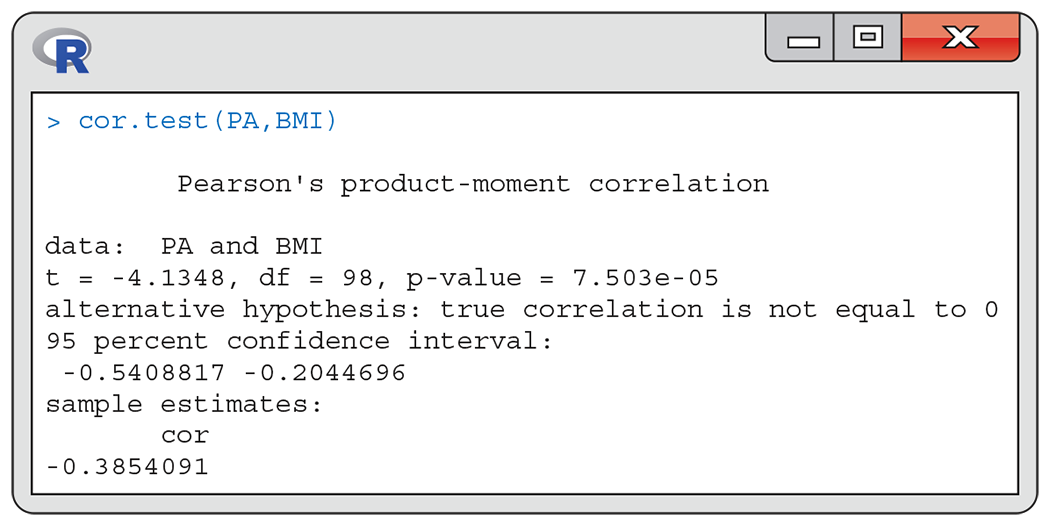
Figure 10.17 R output for the physical activity study, Example 10.23.
To test the one-sided alternative that the population correlation is negative, we divide the P-value in the output by 2, after checking that the sample coefficient is in fact negative. If your software does not give the significance test, you can do the computations easily with a calculator.
Example 10.24 Correlation test using a calculator.
The correlation between BMI and PA is
The degrees of freedom are
There is a close connection between the significance test for a correlation and the test for the slope in a linear regression. Recall that
From this fact we see that if the slope is 0, so is the correlation
and vice versa. It should come as no surprise that the procedures for
testing
In our example the conclusion that there is a statistically
significant correlation between the two variables would not come as a
surprise to anyone familiar with the meaning of these variables. The
significance test simply tells us whether there is evidence in the
data to conclude that the population correlation is different from 0.
The actual size of the correlation is of considerably more interest.
We would therefore like to give a confidence interval for the
population correlation. In
Figure 10.17, R reports a
95% confidence interval for
Check-in
-
10.12 Testing the correlation. The gestational age study of Example 10.16 reports a correlation of
-
Test whether the population correlation is significantly different from zero, using the 0.05 significance level.
-
Compare your t statistic for
-
Section 10.2 SUMMARY
-
Analysis of variance (ANOVA) for simple linear regression partitions the total variation in the responses between two sources: the linear relationship of y with x and the residual variation in responses for the same x.
-
An ANOVA table for a linear regression organizes these ANOVA calculations into degrees of freedom, sums of squares, and mean squares for the model, error, and total sources of variation. The ANOVA F statistic is the ratio MSM/MSE. Under
-
The square of the sample correlation can be expressed as
and is interpreted as the proportion of the variability in the response variable y that is explained by the explanatory variable x in the linear regression.
-
The standard errors for
-
The standard error of
This standard error is used in a confidence interval.
-
The standard error for predicting an individual response
This standard error is used in a prediction interval.
-
When the variables y and x are jointly Normal, the sample correlation is an estimate of the population correlation
which has a
Section 10.2 EXERCISES
-
10.19 What’s wrong? For each of the following, explain what is wrong and why.
-
In simple linear regression, the null hypothesis of the ANOVA F test is
-
In an ANOVA table, the mean squares add. In other words,
-
The smaller the P-value for the ANOVA F test, the greater the explanatory power of the model.
-
The total degrees of freedom in an ANOVA table are equal to the number of observations n.
-
-
10.20 What’s wrong? For each of the following, explain what is wrong and why.
-
In simple linear regression, the standard error for a future observation is s, the measure of spread about the regression line.
-
In an ANOVA table, SSE is the sum of the deviations.
-
There is a close connection between the correlation r and the intercept of the regression line.
-
The squared correlation
-
-
10.21 Research and development spending. The National Science Foundation collects data on research and development spending by universities and colleges in the United States.11 Here are the data for spending in the years 2013–2016 that was nonfederally funded:
Year 2013 2014 2015 2016 Spending (billions of dollars) 27.6 29.2 30.7 33.0 Do the following by hand or with a calculator and verify your results with a software package or Excel.

-
Create a scatterplot that shows the increase in research and development spending over time. Does the pattern suggest that the spending is increasing linearly over time? Explain your answer.
-
Find the equation of the least-squares regression line for predicting spending over time. Add this line to your scatterplot.
-
For each of the four years, find the residual. Use these residuals to calculate the regression standard error s.
-
Write the regression model for this setting. What are your estimates of the unknown parameters in this model?
-
Use your least-squares results to construct a 95% prediction interval for research and development spending for 2017. The actual spending for that year was $34.9 billion. Comment on how well the model predicted the actual outcome.
-
Explain why a prediction interval rather than a confidence interval is appropriate for part (e).
(Comment: These are time series data. Simple regression is often a good fit to time series data over a limited span of time.)
-
-
10.22 Food neophobia. Food neophobia is a personality trait associated with avoiding unfamiliar foods. In one study of 564 children who were two to six years of age, the degree of food neophobia and the frequency of consumption of different types of food were measured.12 Here is a summary of the correlations:
Type of food Correlation Vegetables Fruit Meat Eggs Sweet/fatty snacks 0.04 Starchy staples Perform the significance test for each correlation and write a summary about food neophobia and the consumption of different types of food.
-
10.23 Correlation between the prevalences of adult binge drinking and underage drinking. A group of researchers compiled data on the prevalence of adult binge drinking and the prevalence of underage drinking in 42 states.13 A correlation of 0.32 was reported.
-
Test the null hypothesis that the population correlation
-
Explain this correlation in terms of the direction of the association and the percent of variability in the prevalence of underage drinking that is explained by the prevalence of adult binge drinking.
-
The researchers collected information from 42 of 50 states, so almost all the data available were used in the analysis. Provide an argument for the use of statistical inference in this setting.
-
-
10.24 Grade inflation. The average undergraduate GPA for American colleges and universities was estimated based on a sample of institutions that published this information.14 Here are the data for public schools in that report:
Year 1992 1996 2002 2007 GPA 2.85 2.90 2.97 3.01 Do the following by hand or with a calculator and verify your results with a software package.

-
Make a scatterplot that shows the increase in GPA over time. Does a linear increase appear reasonable?
-
Find the equation of the least-squares regression line for predicting GPA from year. Add this line to your scatterplot.
-
Compute a 95% confidence interval for the slope and summarize what this interval tells you about the increase in GPA over time.
-
-
10.25 Completing an ANOVA table. How are returns on common stocks in overseas markets related to returns in U.S. markets? Consider measuring U.S. returns by the annual rate of return on the Standard & Poor’s 500 stock index and overseas returns by the annual rate of return on the Morgan Stanley Europe, Australasia, Far East (EAFE) index.15 Both are recorded in percents. We will regress the EAFE returns on the S&P 500 returns for the 31 years 1989 to 2019. Here is part of the Minitab output for this regression:
The regression equation isEAFE = −3.50 + 0.831 S&PAnalysis of VarianceSource DF SS MS FRegression 1 6427.4Residual ErrorTotal 11108.5Using the ANOVA table format on page 543 as a guide, complete the analysis of variance table.
-
10.26 Interpreting statistical software output. Refer to the previous exercise. What are the values of the estimated model standard error s and the squared correlation
-
 10.27 Confidence intervals for the slope and intercept.
Refer to the previous two exercises. The mean and standard
deviation of the S&P 500 returns for these years are 12.11%
and 17.61%, respectively. From this and your work in the
previous two exercises:
10.27 Confidence intervals for the slope and intercept.
Refer to the previous two exercises. The mean and standard
deviation of the S&P 500 returns for these years are 12.11%
and 17.61%, respectively. From this and your work in the
previous two exercises:
-
Find the standard error for the least-squares slope
-
Give a 95% confidence interval for the slope
-
Explain why the intercept
-
Find the standard error for the least-squares intercept
-