13.2 Inference for Two-Way ANOVA in Chapter 13 Two-Way Analysis of Variance

13.2 Inference for Two-Way ANOVA

Because two-way ANOVA breaks the FIT part of the model into three parts, corresponding to the two main effects and the interaction, inference for two-way ANOVA includes an F statistic for each of these effects. As with one-way ANOVA, the calculations are organized in an ANOVA table.

The two-way ANOVA table

The results of a two-way ANOVA are summarized in an ANOVA table based on splitting the total variation SST and the total degrees of freedom DFT among the two main effects, the interaction, and error. When the sample size is the same for all cells, both the sums of squares and the degrees of freedom add:

SST=SSA+SSB+SSAB+SSEDFT=DFA+DFB+DFAB+DFE

caution When the nij are not all equal, there are different ways to break down SST, and some can give sums of squares that do not add. The degrees of freedom, on the other hand, will always add.

For this chapter, we consider inference only for the equal-sample-size case. When the nij vary, the choice of SST breakdown and, therefore, the resulting interpretations of the F tests vary. When the counts are approximately equal, all breakdowns give essentially the same results. Thus, to avoid these complications, try to design studies with equal sample sizes whenever possible. If the nij vary quite a bit, either by design or because of dropouts, seek an expert to explain these different SST breakdowns.

From each sum of squares and its degrees of freedom, we find the mean square in the usual way:

mean square=sum of squaresdegree of freedom

The significance of each of the main effects and the interaction is assessed by an F statistic that compares the variation due to the effect of interest with the within-group variation. Each F statistic is the mean square for the source of interest divided by MSE.

Here is the general form of the two-way ANOVA table:

Source	Degrees of freedom	Sum of squares	Mean square	F
A	I−1	SSA	SSA/DFA	MSA/MSE
B	J−1	SSB	SSB/DFB	MSB/MSE
AB	(I−1)(J−1)	SSAB	SSAB/DFAB	MSAB/MSE
Error	N−IJ	SSE	SSE/DFE
Total	N−1	SST

There are three null hypotheses in two-way ANOVA, with an F test for each. We can test for significance of the main effect of A, the main effect of B, and the AB interaction. caution It is generally good practice to examine the test for interaction first because the presence of a strong interaction may influence the interpretation of the main effects. Be sure to plot the means as an aid to interpreting the results of the significance tests.

Significance tests in two-way ANOVA

To test the main effect of A, use the F statistic

FA=MSAMSE

To test the main effect of B, use the F statistic

FB=MSBMSE

To test the interaction of A and B, use the F statistic

FAB=MSABMSE

If the variation due to the effect being tested is zero, the F statistic has an F distribution with numerator degrees of freedom corresponding to that effect and denominator degrees of freedom equal to DFE. The P-value is the probability that a random variable having the corresponding F distribution is greater than or equal to the calculated value. Thus, large values of the F statistic lead to rejection of the null hypothesis.

Recall that these F tests and resulting P-values can be trusted only if the model conditions are approximately met. The two-way ANOVA model conditions are the same as those for the one-way ANOVA with IJ groups, so we use the same methods to check these conditions.

Check-in

13.5 Haptic feedback and difficulty level. Example 13.2 (page 652) describes the setting for a two-way ANOVA design that compares different types of controllers and obstacle course difficulty levels. Give the degrees of freedom for each of the F statistics that are used to test the main effects and the interaction for this problem.
13.6 The effect of a limited-time offer. Exercise 13.3 (page 653) describes the setting for a two-way ANOVA design that tests the effect of the phrase “limited-time offer” in two types of consumers. Give the degrees of freedom for each of the F statistics that are used to test the main effects and the interaction for this problem.

Carrying out a two-way ANOVA

Data set icon for Vtm.

The following example illustrates how to do a two-way ANOVA. As with the one-way ANOVA, we focus our attention on interpretation of software output.

Example 13.8 A study of cardiovascular risk factors.

Data set icon for hrtrate.

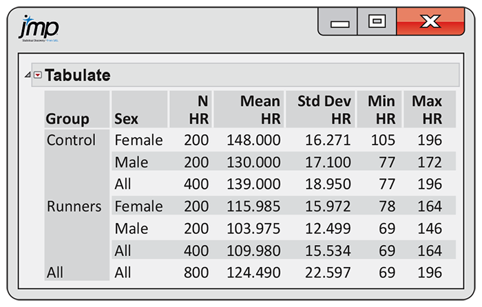
A study of cardiovascular risk factors compared runners who averaged at least 15 miles per week with a control group described as “generally sedentary.” Both men and women were included in the study.¹⁰ The design is a 2×2 ANOVA with the factors Group and Sex. There were 200 subjects in each of the four combinations. One of the variables measured was the heart rate after six minutes of exercise on a treadmill. JMP produced the outputs in Figure 13.5 and Figure 13.6.

A JMP output of a summary statistics table. — Figure 13.5 Summary statistics for the heart-rate study, Example 13.8.

The output shows an expanded dropdown list menu, tabulate, which shows a table of data. A table has 7 rows and 7 columns. The columns have the following headings from left to right. Group, Sex, N H R, Mean H R, Standard deviation H R, Minimum H R, Maximum H R, . The row entries are as follows. Row 1. Group, Control. Sex, Female. N H R, 200. Mean H R, 148. Standard deviation H R, 16.271. Minimum H R, 105. Maximum H R, 196. Row 2. Group, Control. Sex, Male. N H R, 200. Mean H R, 130. Standard deviation H R, 17.1. Minimum H R, 77. Maximum H R, 172. Row 3. Group, Control. Sex, All. N H R, 400. Mean H R, 139. Standard deviation H R, 18.95. Minimum H R, 77. Maximum H R, 196. Row 4. Group, Runners. Sex, Female. N H R, 200. Mean H R, 115.985. Standard deviation H R, 15.972. Minimum H R, 78. Maximum H R, 164. Row 5. Group, Runners. Sex, Male. N H R, 200. Mean H R, 103.975. Standard deviation H R, 12.499. Minimum H R, 69. Maximum H R, 146. Row 6. Group, Runners. Sex, All. N H R, 400. Mean H R, 109.98. Standard deviation H R, 15.534. Minimum H R, 69. Maximum H R, 164. Row 7. Group, All. Sex, All. N H R, 800. Mean H R, 124.49. Standard deviation H R, 22.597. Minimum H R, 69. Maximum H R, 196.

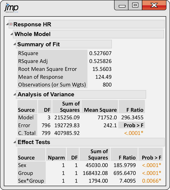
A JMP output of a two-way ANOVA analysis. — Figure 13.6 Two-way ANOVA output for the heart-rate study, Example 13.8.

The output shows three expanded dropdown list menus, response H R, whole model, and summary of fit. Below is a table with the following data. R square, 0.527607. R square adjusted, 0.525826. Root mean square error, 15.5603. Mean of response, 124.49. Observations, or sum weights, 800. Another expanded menu, analysis of variance, shows a table with the following data. Source, model. D F, 3. Sum of squares, 215256.09. Mean square, 71752.0. F ratio, 296.3455. Source, error. D F, 796. Sum of squares, 192729.83. Mean square, 242.1. Source, C total. D F, 799. Sum of squares, 407985.92. Probability greater than F, less than 0.0001 asterisk. Another expanded menu, effect tests, shows a table with the following data. Source, sex. N parm, 1. D F, 1. Sum of squares, 45030.00. F ratio, 185.9799. Probability greater than F, less than 0.0001 asterisk. Source, group. N parm, 1. D F, 1. Sum of squares, 168432.08. F ratio, 695.6470. Probability greater than F, less than 0.0001 asterisk. Source, sex times group. N parm, 1. D F, 1. Sum of squares, 1794.00. F ratio, 7.4095. Probability greater than F, 0.0066 asterisk.

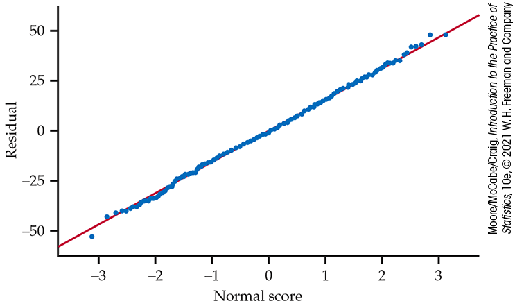
We begin with the usual preliminary examination of model conditions. From Figure 13.5, we see that the ratio of the largest to the smallest standard deviation in the four cells (17.10/12.499=1.37) is less than 2. Therefore, we are not concerned about violating the assumption of equal population standard deviations. The Normal quantile plot in Figure 13.7 suggests that the deviations are reasonably Normal, with no outliers.

A normal quantile plot. — Figure 13.7 Normal quantile plot for the heart-rate study, Example 13.8.

The ANOVA table in the middle of the output in Figure 13.6 is, in effect, a one-way ANOVA with four groups: female control, female runner, male control, and male runner. In this analysis, Model has 3 degrees of freedom, and Error has 796 degrees of freedom. Because we will be relying on software to do all these calculations, it is a good idea to do some quick arithmetic checks like degrees of freedom to make sure things make sense. The F test and its associated P-value for this analysis refer to the hypothesis that all four groups have the same population mean. We are interested in the main effects and interaction, so we ignore this test here.

Two-way ANOVA splits the variation among the means (expressed by the Model sum of squares) into three parts that reflect the two-way layout. The sums of squares for the Sex and Group main effects and the Sex-by-Group interaction appear at the bottom of Figure 13.6, under the heading “Effect Tests.” These sum to the sum of squares for Model. Similarly, the degrees of freedom for these sums of squares sum to the degrees of freedom for Model.

Because the degrees of freedom are all 1 for the main effects and the interaction, the mean squares (not shown in the JMP output) are the same as the sums of squares. The F statistics for the three effects appear in the column labeled “F Ratio,” and the P-values are under the heading “Prob > F.” For the Group main effect, we verify the calculation of F as follows:

F=MSGMSE=168,432242.12=695.65

All three effects are statistically significant. The Group effect has the largest F, followed by the Sex effect and then the Sex-by-Group interaction. To interpret these results, we examine the interaction plot, with bars indicating the 95% confidence interval for each group mean, in Figure 13.8. Note that the confidence intervals are quite narrow because of the large sample sizes.

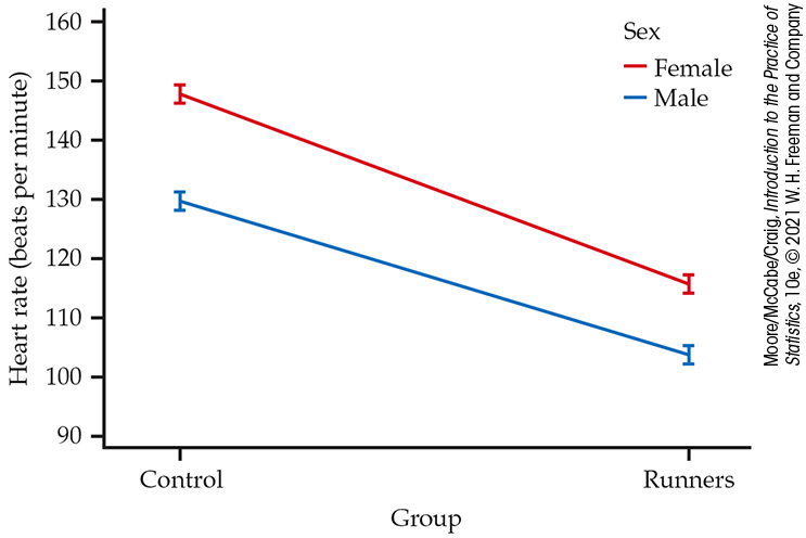
An interaction plot heart rate versus group. — Figure 13.8 Interaction plot of heart-rate study with 95% confidence intervals for the means indicated, Example 13.8.

The graph plots heart rate in beats per minute on the vertical axis, ranging from 90 to 160 in increments of 10, versus group on the horizontal axis, with two groups listed, control and runner. The graph shows two plots for female and male. Each sex has a confidence interval plotted for each group, with a line falling between the center of them. By sex, the confidence intervals are as follows. Female. Control. Lower, 146. Upper, 150. Runners. Lower, 115. Upper, 119. The plot falls from (control, 148) to (runners, 117). Male. Control. Lower, 128. Upper, 132. Runners. Lower, 103. Upper, 107. The plot falls from (control, 130) to (runners, 105). All values estimated.

The significance of the main effect for Group is due to the fact that the controls have higher average heart rates than the runners for both sexes. We can describe this main effect using the marginal means for Group presented in Figure 13.5. Their difference is 139.00−109.98=29.02 beats. This is the largest effect evident in the plot.

The significance of the main effect for Sex is due to the fact that the females have higher heart rates than the males in both groups. We can use the cell means in Figure 13.5 to describe this main effect. The difference in marginal means is

148.000+115.9852+130.000+103.9752=15.01

beats. This difference is smaller than that for Group, and this is reflected in the smaller value of the F statistic.

The analysis also indicates that a complete description of the average heart rates requires consideration of the interaction in addition to the main effects (P=0.0066). The two lines in the interaction plot are not parallel, and the gap between males and females is slightly larger in the control group. This interaction can be described in two ways. The female/male difference in average heart rates is greater for the controls than for the runners. Alternatively, the difference in average heart rates between controls and runners is greater for women than for men.

As the plot suggests, the interaction is not large. The difference between the sexes in the control group is 18 beats per minute, and the difference between the sexes in the runners group is 12 beats per minute. The fact that these deviations from the main effect of 15 beats are so highly statistically significant is largely because there were 800 subjects in the study. Our estimate of the common group standard deviation is

sp=MSE=15.56

meaning deviations of ±3 beats is slightly less than one-fifth of a standard deviation. The researchers may or may not consider this interaction of practical value.

Two-way ANOVA output for other software is similar to that given by JMP. Figure 13.9 gives the analysis of the heart rate data using Excel and Minitab.

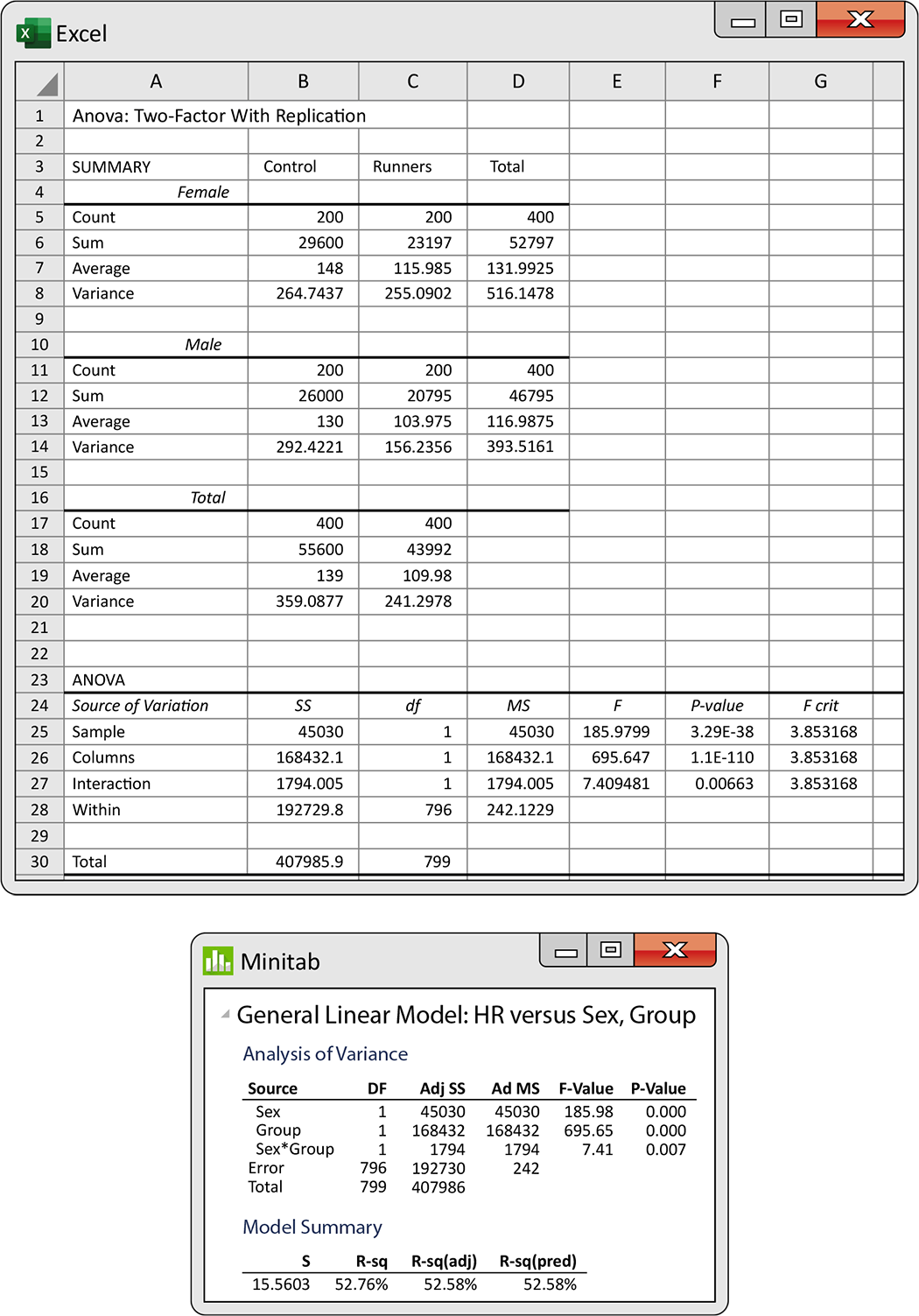
Excel and Minitab outputs for an ANOVA analysis. — Figure 13.9 Excel and Minitab analysis of variance outputs for the heart-rate study, Example 13.8.

The Excel output is titled, ANOVA, two-factor with replication. It shows four tables of data as follows. Summary. First table, female. Item, count. Control, 200. Runners, 200. Total, 400. Item, sum. Control, 29600. Runners, 23197. Total, 52797. Item, average. Control, 148. Runners, 115.985. Total, 131.9925. Item, variance. Control, 264.7437. Runners, 255.0902. Total, 516.1478. Second table, male. Item, count. Control, 200. Runners, 200. Total, 400. Item, sum. Control, 26000. Runners, 20795. Total, 46795. Item, average. Control, 130. Runners, 103.975. Total, 116.9875. Item, variance. Control, 292.4221. Runners, 156.2356. Total, 393.5161. Third table, total. Item, count. Control, 400. Runners, 400. Item, sum. Control, 55600. Runners 43992. Item, average. Control, 139. Runners, 109.98 2. Item, variance. Control, 359.0877. Runners, 241.2978. Fourth table, ANOVA. Source of variation, sample. S S, 45030. d f, 1. M S, 45030. F, 185.9799. P-value, 3.29 E negative 38. F critical, 3.853168. Source of variation, columns. S S, 168432.1. d f, 1. M S, 168432.1. F, 695.647. P-value, 1.1 E negative 10. F critical, 3.853168. Source of variation, interaction. S S, 1794.005. d f, 1. M S, 1794.005. F, 7.409481. P-value, 0.00663. F critical, 3.853168. Source of variation, within. S S, 192729.8. d f, 796. M S, 242.1229. Source of variation, total. S S, 407985.9. d f, 799. The Minitab output is titled, general linear model, H R versus sex, group. It shows two tables of data as follows. First table, analysis of variance. Source, sex. D F, 1. Adjusted S S, 45030. Adjusted M S, 45030. F-value, 185.98. P-value, 0.000. Source, group. D F, 1. Adjusted S S, 168432. Adjusted M S, 168432. F-value, 695.65. P-value, 0.000. Source, sex times group. D F, 1. Adjusted S S, 1794. Adjusted M S, 1794. F-value, 7.41. P-value, 0.000. Source, error. D F, 796. Adjusted S S, 192730. Adjusted M S, 242. Source, total. D F, 799. Adjusted S S, 407986. Second table, model summary. S, 15.5603. R square, 52.76 percent. R square adjusted, 52.58 percent. R square predicted, 52.58 percent.

Section 13.2 SUMMARY

Prior to inference, the two-way ANOVA model conditions should be assessed. These conditions are the same as those for the one-way ANOVA model. A comparison of standard deviations as well as a histogram or Normal quantile plot of the residuals can help in determining whether the conditions are approximately met.
The calculations for two-way ANOVA are organized into a two-way ANOVA table. The key difference from one-way ANOVA is that the group variation is separated into parts for the main effect of each factor and the interaction of the factors.
When the sample size is the same for all cells, both the sums of squares and the degrees of freedom add:

SST=SSA+SSB+SSAB+SSEDFT=DFA+DFB+DFAB+DFE

Here A and B refer to the main effects of the two factors, and AB refers to the interaction.
F statistics and P-values are used to test hypotheses about the main effects and the interaction. Under the null hypothesis, each F statistic has an F distribution with numerator degrees of freedom corresponding to the effect being tested and denominator degrees of freedom equal to DFE.

Now that you have completed this section, you will be able to:

Construct the two-way ANOVA table in terms of sources and degrees of freedom. Review page 664 and try Exercise 13.15.
Summarize how to use the two-way ANOVA table F tests to assess the statistical significance of main effects interaction. Review pages 664–665 and try Exercises 13.19 and 13.21.
Interpret software output for a two-way ANOVA. Review Example 13.8 (page 665) and try Exercises 13.23.
Use software to generate diagnostic plots and numerical summaries to check the ANOVA conditions for valid inference. Review pages 666–667 and try Exercise 13.23.

Section 13.2 EXERCISES

13.12 How large does the F statistic need to be? For each of the following situations, sketch the F distribution and indicate the region where you would reject at the 5% significance level.
1. The main effect for B in a 2×4 ANOVA with three observations per cell.
2. The interaction in a 4×3 ANOVA with six observations per cell.
3. The main effect for A in a 3×3 ANOVA with four observations per cell.
13.13 What’s wrong? For each of the following, explain what is wrong and why.
1. For a 3×5 ANOVA, DFAB=15.
2. You can perform a two-way ANOVA only when the sample sizes are the same in all cells.
3. In a two-way ANOVA, the error variation is separated in parts for each main effect and interaction.
4. In a 2×3 ANOVA, we compare the means of five groups.
13.14 Outlining the ANOVA table. For each part in Exercise 13.3 (page 661), outline the ANOVA table, giving the sources of variation and the degrees of freedom.
13.15 Is there interaction? A 3×3 ANOVA was run with four observations per cell.
1. Outline the two-way ANOVA table for this analysis, giving the sources of variation and the degrees of freedom.
2. Give the degrees of freedom for the F statistic that is used to test for interaction in this analysis and the entries from Table E that correspond to this distribution.
3. Sketch a picture of this distribution with the information from the table included.
4. The calculated value of this F statistic is 3.03. Report the P-value and state your conclusion.
5. Based on your answer to part (c), would you expect an interaction plot to have mean profiles that look parallel? Explain your answer.

13.16 What can you conclude, given the P-values? A study reported the following results for data analyzed using a two-way ANOVA at the 5% significance level:

Effect	F	P-value
A	4.75	0.009
B	14.26	0.001
AB	5.14	0.007

What can you conclude from the information given?
What additional information would you need to write a summary of the results for this study?

13.17 What can you conclude, given the design and F statistics? Analysis of data for a 2×3 ANOVA with five observations per cell gave the following F statistics:

Effect	F
A	3.28
B	4.64
AB	1.43

What can you conclude from the information given?
What additional information would you want in order to write a complete summary?

13.18 Ecological effects of pharmaceuticals on fish. Drugs used to treat anxiety persist in wastewater effluent, resulting in relatively high concentrations of these drugs in our rivers and streams. To understand the impacts of these anxiety drugs on fish, researchers commonly expose fish to various levels of a drug in a laboratory setting and observe their behavior.¹¹ In one 2×2 experiment, researchers considered exposure to oxazepan through the water (Y/N) and through the diet (Y/N). Ten one-year-old perch were assigned to each of the four treatment combinations. After seven days of exposure, each fish was observed for activity. This was recorded as the number of swimming bouts (defined as movement exceeding 3.5 cm) over a 10-minute period.
1. The response is the number of movements in 10 minutes, which can only be a whole number. Should we be concerned about violating the assumption of Normality? Explain your answer.
2. Construct an interaction plot and comment on the main effects of exposure through diet and water and their interaction.
3. Analyze the count of swimming bouts using analysis of variance. Report the test statistics, degrees of freedom, and P-values.
4. Use the residuals to check the model assumptions. Are there any concerns? Explain your answer.
5. Based on parts (c) and (d), write a short paragraph summarizing your findings.

13.19 Study of resveratrol and dietary copper. Past studies have shown that cardiovascular alterations can be improved through long-term use of dietary copper and resveratrol. A study in rats was run to look at the interaction between resveratrol and two forms of copper. This experiment involved 36 rats, equally divided among four groups. The four groups were carbonate copper or nanoparticle copper, each with and without resveratrol. After eight weeks of supplementation, the rats were sacrificed, and various outcomes were measured.¹² The partial output in the following ANOVA table summarizes the content of glucose in the blood at the time of sacrifice:

Source	Sum of squares	Mean square
Copper	7.13
Resveratrol	22.75
Interaction	29.81
Error		6.71
Total

Fill in the missing entries in the ANOVA table.
What is sp, the pooled standard error?
What is the coefficient of determination R2 for this study?
State H0 and Ha for each of the F tests in this analysis.
Using Table E (or software), give an approximate (exact) P-value for each test.
Write a brief conclusion of what you find.

13.20 Ecological effects of pharmaceuticals on fish (continued). Refer to Exercise 13.18.
1. Often with a count as the response, one considers taking the square root of the count and performing ANOVA on this transformed response. Explain why a transformation might be useful here.
2. Using the response SqrtCnt, repeat parts (b) through (e) of Exercise 13.18.
3. Which analysis do you prefer here? Explain your answer.

13.21 Study of resveratrol and dietary copper (continued). Refer to Exercise 13.19. The mean glucose level (mmol/L) for each group of rats is shown in the following table:

Group	x¯
Carbonate	17.66
Carbonate + resveratrol	17.89
Nanoparticle	20.37
Nanoparticle + resveratrol	16.96

Construct an interaction plot.
Combine the information in your interaction plot with the conclusions from Exercise 13.19 to better elaborate what this study found.

13.22 Hypotension and endurance exercise. In sedentary individuals, low blood pressure (hypotension) often occurs after a single bout of aerobic exercise and lasts nearly two hours. This can cause dizziness, light-headedness, and possibly fainting upon standing. It is thought that endurance exercise training can reduce the degree of postexercise hypotension. To test this, researchers studied 16 endurance-trained and 16 sedentary men and women.¹³ The following table summarizes the postexercise systolic arterial pressure (mm Hg) after 60 minutes of upright cycling:

Group	n	x¯	SE
Women, sedentary	8	100.7	3.4
Women, endurance	8	105.3	3.6
Men, sedentary	8	114.2	3.8
Men, endurance	8	110.2	2.3

Make a plot similar to Figure 13.3 (page 660) with the systolic blood pressure on the y axis and training level on the x axis. Describe the pattern you see.
From the table, one can show that SSA=677.12, SSB=0.72, SSAB=147.92, and SSE=2478, where A is the sex effect and B is the training level. Construct the ANOVA table with F statistics and degrees of freedom and state your conclusions regarding main effects and interaction.
The researchers also measured the before-exercise systolic blood pressure of the participants and looked at a model that incorporated both the pre- and postexercise values. Explain why it is likely to be beneficial to incorporate both measurements in the study.

13.23 Smart shopping carts. Smart shopping carts are shopping carts equipped with scanners that track the total price of the items in the cart (providing real-time feedback). To help understand the smart shopping cart’s influence on spending behavior, a group of researchers designed a two-factor study. Each participant was randomly assigned to either be on or not on a budget of $35. Also, each participant’s cart was equipped with or not equipped with real-time feedback. The total amount spent on a common grocery list was the response.¹⁴
1. Construct a plot of the means and describe the main features of the plot.
2. Use diagnostic plots and numeric summaries to check ANOVA model conditions.
3. Analyze the data using a two-way ANOVA. Report the F statistics, degrees of freedom, and P-values. Because the nij are not equal, different software may give slightly different F statistics and P-values.
4. Write a short summary of your findings.