13.1 The Two-Way ANOVA Model
In one-way ANOVA, we classify populations according to one categorical variable, or factor. In two-way ANOVA, there are two factors, each with its own number of levels. When we are interested in the effects of two factors, a two-way design offers great advantages. We begin this section with a discussion of these advantages, illustrated through some examples. Then we discuss the two-way ANOVA model and the breakdown of the population means into main effects and interaction.
Advantages of two-way ANOVA
When we are interested in the effects of two factors, a two-way design offers several great advantages over performing two single-factor studies. Each of the following studies highlights one of these advantages.
Example 13.1 Design 1: Does haptic feedback improve performance?
In Example 12.1 (page 600), a group of technology students wanted to see if haptic feedback is helpful in navigating a simulated game environment. To do this, they randomly assigned 20 students to each of three game controller types and recorded the time it took to complete a navigation mission.
It turns out that their simulated game has four difficulty levels. Suppose that a second experiment is planned to compare these levels when using the standard controller. A similar experimental design will be used, with the four difficulty levels randomly assigned equally among the 60 students.
Here is a picture of the designs of the first and second experiments with the sample sizes:
| Controller | n |
|---|---|
| 1 | 20 |
| 2 | 20 |
| 3 | 20 |
| Total | 60 |
| Difficulty | n |
|---|---|
| 1 | 15 |
| 2 | 15 |
| 3 | 15 |
| 4 | 15 |
| Total | 60 |
In the first experiment, 20 students were assigned to each type of game controller, for a total of 60 students. In the second experiment, 15 students were assigned to each level of difficulty, for a total of 60 students. It is expected that each experiment lasts one week, so the total amount of time for the two experiments is two weeks.
Each experiment will be analyzed using one-way ANOVA. The factor in the first experiment is Controller with three levels, and the factor in the second experiment is Difficulty with four levels. Let’s now consider combining the two experiments into one.
Example 13.2 Design 2: Does haptic feedback improve performance regardless of difficulty level?
Suppose that we use a two-way approach for the haptic feedback
study. There are two factors, Controller and Difficulty. Because
Controller has three levels and Difficulty has four levels, this is
a
Here is a picture of the two-way design with the sample sizes:
| Controller | Difficulty | Total | |||
|---|---|---|---|---|---|
| 1 | 2 | 3 | 4 | ||
| 1 | 5 | 5 | 5 | 5 | 20 |
| 2 | 5 | 5 | 5 | 5 | 20 |
| 3 | 5 | 5 | 5 | 5 | 20 |
| Total | 15 | 15 | 15 | 15 | 60 |
Each combination of the factors in a two-way design corresponds to a
cell. The
With the two-way design, notice that we have 20 students assigned to each level of Controller, the same as we had for the one-way experiment for Controller alone. Similarly, there are still 15 students assigned to each level of Difficulty. Thus, the two-way design gives us the same amount of information for estimating the completion time for each level of each factor as we had with the two one-way designs.
The difference is that we can collect all the information in only one experiment. This experiment should last one week (instead of a combined two weeks) and involves a single observation from each of the 60 students. By combining the two factors into one experiment, we have increased our efficiency by reducing the amount of data to be collected by half.
Example 13.3 The effect of a limited time offer on purchase intent.
Starbucks’s Pumpkin Spice Latte (PSL) is the company’s most popular seasonal item. Why is this? Is it the unique flavor? Or could it be because it is available only for a limited time each year? To investigate this, some students surveyed 100 Starbucks consumers about their intent to purchase a PSL when it is offered in the fall.2 Half of the surveys included the upcoming PSL advertisement. The other half included the same advertisement with the additional words “Limited Time Offer” above the image of the drink. Because purchase intent may depend on how frequently a consumer visits Starbucks, the students included a survey question about this. The question was used to classify each customer as either a “light” or “heavy” consumer of Starbucks.
The factors for the two-way ANOVA are advertisement type with two
levels and consumer status with two levels. There are
Here is a table of sample sizes that summarizes the design:
| Advertisement | Consumer status | Total | |
|---|---|---|---|
| Light | Heavy | ||
| Regular | 27 | 23 | 50 |
| Added wording | 19 | 31 | 50 |
| Total | 46 | 54 | 100 |
The students were not able to control the number of subjects in each cell of the study because they did not know consumer status until the survey was administered.
This example illustrates another advantage of two-way designs. Although the students are primarily interested in the effect of adding the words “Limited Time Offer” on purchase intent, they also included consumer status because they suspected that the wording effect might be different in light and heavy consumers.
Consider an alternative one-way design where we ignore consumer
status. With this design, we will have the same number of customers at
each of the advertisement type levels, so in this way, it is similar
to our two-way design. However, suppose that there are, in fact,
differences in outcome due to consumer status. In this case, the
one-way ANOVA would assign this variation to the RESIDUAL (within
groups) part of our conceptual model. In the two-way ANOVA, consumer
status is included as a factor; therefore, this variation is included
in the FIT part of the model.
Whenever we can move variation from RESIDUAL to FIT, we reduce the
Example 13.4 Vitamin D and osteoporosis.

Osteoporosis is a disease primarily affecting elderly individuals. People with osteoporosis have low bone mass and an increased risk of bone fractures. More than 10 million people in the United States, 1.4 million Canadians, and many millions elsewhere throughout the world have this disease. Adequate calcium in the diet is necessary for strong bones, but vitamin D is also needed for the body to efficiently use calcium. High doses of calcium in the diet will not prevent osteoporosis unless there is adequate vitamin D. Exposure of the skin to the ultraviolet rays in sunlight enables our bodies to make vitamin D. However, elderly people often don’t go outside as much as younger people do, and in northern areas such as Canada, there is not sufficient ultraviolet light for the body to make vitamin D, particularly in the winter months.
Suppose that we wanted to see if calcium supplements will increase
bone mass (or prevent a decrease in bone mass) in an elderly
Canadian population. Because of the vitamin D complication, we will
make this a factor in our design. We will use a
Women between the ages of 70 and 80 will be recruited as subjects. Bone mineral density (BMD) will be measured at the beginning of the study, and supplements will be taken for one year. The change in BMD over the one-year period is the outcome variable. We expect a dropout rate of 20%, and we would like to have about 40 subjects providing data in each group at the end of the study. We will, therefore, recruit 200 subjects and randomly assign 50 to each treatment combination.
Here is a table that summarizes the planned design with the sample sizes at the start of the study:
| Calcium | Vitamin D | Total | |
|---|---|---|---|
| Placebo | 300 IU/d | ||
| Placebo | 50 | 50 | 100 |
| 800 mg/d | 50 | 50 | 100 |
| Total | 100 | 100 | 200 |
This example illustrates a third reason for using two-way designs. The effectiveness of the calcium supplement on BMD may differ across the two levels of vitamin D. We call this an interaction. In contrast, the average values for the calcium effect and the vitamin D effect are represented as main effects. The two-way model represents FIT as the sum of a main effect for each of the two factors and an interaction. One-way designs that vary a single factor and hold other factors fixed cannot discover interactions. We will discuss interactions more fully later in this section.
These examples illustrate three reasons two-way designs are preferable to one-way designs.
These considerations also apply to study designs with more than two
factors. The statistical analysis in these situations is broadly
called
higher-way
ANOVA. Although some details grow more complex, the most important ideas
are already present in the two-way setting. Thus, we will be content
to explore only the two-way case. Remember that the choice of sampling
or experimental design is fundamental to any statistical study.
![]() Factors and levels must be carefully selected by an individual or a
team who understands both the statistical models and the issues that
the study will address.
Factors and levels must be carefully selected by an individual or a
team who understands both the statistical models and the issues that
the study will address.
The two-way ANOVA model
When discussing two-way models in general, we will use the labels A and B for the two factors. For particular examples and when using statistical software, it is better to use meaningful names for these categorical variables. Thus, in Example 13.2 (page 652), we would say that the factors are Controller and Difficulty, and in Example 13.4, we would say that the factors are Calcium and Vitamin D.
The numbers of levels of the factors are often used to describe the
model. Again using our earlier examples, we would say that
Example 13.2
represents a
In a two-way design, every level of A appears in combination with
every level of B, so that
Much as in the one-way model, the FIT part is the group means
The k below the
The RESIDUAL part of the model is represented by the unknown
Just as in one-way ANOVA, the numerator in this fraction is SSE, and
the denominator is DFE. Also, DFE is the total number of observations
minus the number of groups. That is,
Check-in
-
13.1 Limited-time offer effect on purchase intent. Example 13.3 (page 653) describes a study designed to compare different advertisement types and consumer status on purchase intent. Write out the ANOVA model for this study. Be sure to give specific values for I, J, and
-
13.2 Limited-time offer effect on purchase intent (continued). Refer to the previous Check-in question. The following table summarizes the group means and standard deviations:
Consumer Advertisement s Light Regular 4.56 1.75 Light Added wording 5.74 1.19 Heavy Regular 5.00 1.79 Heavy Added wording 5.19 1.91 -
Is it reasonable to pool the standard deviations for these data? Explain your answer.
-
For each parameter in your model from the previous Check-in question, give the estimate.
-
Main effects and interactions
So far, we have presented the two-way ANOVA as a one-way ANOVA with
IJ groups. Each population mean
Because the two-way model gives some structure to the group means
and
The term SSA represents variation among the means for the different
levels of Factor A. Because there are I such means,
Interactions are a bit more involved. We can see that SSAB, which is
There are many kinds of interactions. The easiest way to study them is through examples.
Example 13.5 Investigating differences in sugar-sweetened beverage consumption.
Consumption of sugar-sweetened beverages has been linked to Type 2 diabetes and obesity. One study used data from the National Health and Nutrition Examination Survey (NHANES) to estimate consumption of these beverages. More than 57,000 individuals provided data for this study. Individuals were divided into three age groups: preadolescents (6 to 11 years), adolescents (12 to 19 years), and adults (over 19 years).4 Here are the means for the numbers of calories in sugar-sweetened beverages consumed per day during 2010 and 2016:
| Age group | Year | Mean | |
|---|---|---|---|
| 2010 | 2016 | ||
| Preadolescents | 108.4 | 91.1 | 99.8 |
| Adolescents | 199.1 | 120.5 | 159.8 |
| Adults | 121.8 | 95.2 | 108.5 |
| Mean | 143.1 | 102.3 | 122.7 |
The table in Example 13.5 includes averages of the means in the rows and columns. For example, in 2010 the mean calories consumed per day is
Similarly, the corresponding value for 2016 is
which is rounded to 102.3 in the table. These averages are called marginal means because of their location at the margins of the table. The grand mean (122.7 in this case) can be obtained by averaging either set of marginal means or the six cell means.
It is clear from the marginal means that individuals consumed more
calories from sugar-sweetened beverages in 2010 than in 2016 and that
adolescents consumed more than preadolescents and adults. These are
the main effects for the two factors. We describe them using
differences between marginal means. For example, the main effect of
year going from 2010 to 2016 is a reduction of
What about the interaction between year and age group?
An interaction is present when the marginal means do not tell the
whole story—that is, when the difference between years varies across age groups.
With these data, the marginal mean difference between years is 40.8
calories. This is smaller than the reduction in calories for the
adolescents group
Figure 13.1 is a plot of the group means, where the levels of one factor is used on the x axis and the levels of the other factor are used to connect the means in the plot. This is called an interaction plot because it is a very helpful visual tool to assess and describe main effects and interaction.
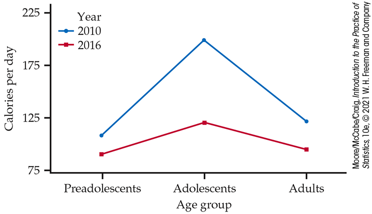
Figure 13.1 Interaction plot of the mean calories per day from sugar-sweetened beverages in 2010 and 2016 for three different age groups, Example 13.5.
From the plot, we see that fewer calories from sugar-sweetened beverages were consumed by each group in 2016 than in 2010. In other words, the 2010 profile, or set of means, is above the 2016 profile. In each profile, we also see that the mean goes up going from preadolescents to adolescents and then down going from adolescents to adults. These patterns are summarizing the main effects.
For interaction, we need to compare profiles. The gap between profiles in Figure 13.1 represents the difference between years for each age group. It is clearly visible that the gap between profiles at the adolescents level is much bigger than the gap at the other two age groups. This suggests that there is interaction.
Check-in
-
13.3 The other interaction plot. The other way to construct the interaction plot for Example 13.5 is to use the levels of year on the x axis and use the levels of age group to connect the means. This will result in three profiles of two means each. Construct this plot using the means in Example 13.5. Do you also see the interaction in this new interaction plot? Explain your answer.
-
13.4 Choosing the better interaction plot. In a two-way ANOVA, there are always two versions of the interaction plot. Choosing which version better describes the important patterns in the data is left to the user. Compare the interaction plot that you constructed in the previous Check-in question with the one in Figure 13.1. Which do you think better describes the important patterns? Explain your answer.
Interaction plots are so helpful in assessing interaction that we recommend all analyses should begin with a plot similar to Figure 13.1. When no interaction is present, the marginal means provide a reasonable description of the two-way table of means. This will be reflected in the plot by profiles that are roughly parallel. If the profiles are not parallel, then an interaction is present.
Interactions come in many shapes and forms.
![]() When we find an interaction, a careful examination of the means is
needed to properly interpret the data. Simply stating that the interaction is significant tells us very
little. Including an interaction plot, on the other hand, helps
immensely with this interpretation.
When we find an interaction, a careful examination of the means is
needed to properly interpret the data. Simply stating that the interaction is significant tells us very
little. Including an interaction plot, on the other hand, helps
immensely with this interpretation.
Example 13.6 Eating in groups.
Some research has shown that people eat more when they eat in groups. One possible mechanism for this phenomenon is that they may spend more time eating when in a larger group. A study designed to examine this idea measured the length of time spent (in minutes) eating lunch in different settings.5 Here are some data from this study:
| Lunch setting | Number of people eating | Mean | ||||
|---|---|---|---|---|---|---|
| 1 | 2 | 3 | 4 | 5 or more | ||
| Workplace | 12.6 | 23.0 | 33.0 | 41.1 | 44.0 | 30.7 |
| Fast-food restaurant | 10.7 | 18.2 | 18.4 | 19.7 | 21.9 | 17.8 |
| Mean | 11.6 | 20.6 | 25.7 | 30.4 | 32.9 | 24.2 |
Figure 13.2 gives the plot of the means for this example. The profiles are not parallel, so it appears that we have an interaction. Meals take longer when there are more people present, but this phenomenon is much greater for the meals consumed at work. For fast-food eating, the meal durations are fairly similar when there is more than one person present.
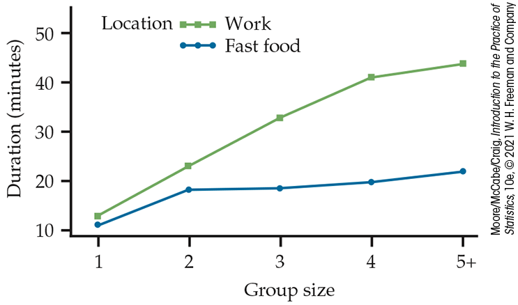
Figure 13.2 Interaction plot of mean meal duration versus lunch setting and group size, Example 13.6.
A different kind of interaction is present in the next example. Here, we must be very cautious in our interpretation of the main effects because either one of them can lead to a distorted conclusion.
Example 13.7 We got the beat?
When we hear music that is familiar to us, we can quickly pick up the beat, and our mind synchronizes with the music. However, if the music is unfamiliar, it takes us longer to synchronize. In a study that investigated the theoretical framework for this phenomenon, French and Tunisian nationals listened to French and Tunisian music.6 Each subject was asked to tap in time with the music being played. A synchronization score, recorded in milliseconds, measured how well the subjects synchronized with the music. A higher score indicates better synchronization. Six songs of each music type were used. Here are the means:
| Nationality | Music | Mean | |
|---|---|---|---|
| French | Tunisian | ||
| French | 950 | 750 | 850 |
| Tunisian | 760 | 1090 | 925 |
| Mean | 855 | 920 | 887 |
The means are plotted in Figure 13.3. In the study, the researchers were not interested in main effects. Their theory predicted the interaction that we see in the figure. Subjects synchronize better with music from their own culture. The main effects, on the other hand, suggest that Tunisians sychronize better than the French (regardless of music type) and that it is easier to synchronize to Tunisian music (regardless of nationality).
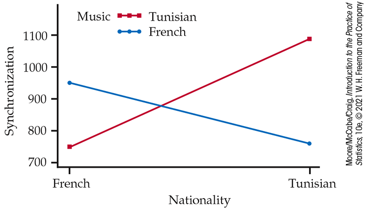
Figure 13.3 Plot of mean synchronization score versus type of music for French and Tunisian nationals, Example 13.7.
The interaction in Figure 13.3 is very different from the interactions we saw in Figures 13.1 and 13.2. These examples illustrate the point that it is necessary to plot the means and carefully describe the patterns when interpreting an interaction.
The design of the study in
Example 13.7
allows us to examine two main effects and an interaction. However,
this setting does not meet all the assumptions needed for statistical
inference using the two-way ANOVA framework of this chapter.
![]() As with one-way ANOVA, we require that observations be
independent.
As with one-way ANOVA, we require that observations be
independent.
In this study, we have a design that has each subject contributing data for two types of music, so these two scores will be dependent. The framework is similar to the matched pairs design. This design is called a repeated-measures design. More advanced texts on statistical methods cover this important design.
Section 13.1 SUMMARY
-
Two-way ANOVA is used to compare population means when populations are classified according to two factors. When interested in the effects of two factors, it is more efficient to analyze the factors simultaneously. This also allows you to investigate interaction.
-
Each combination of factors in a two-way design corresponds to a cell. In an
-
The two-way ANOVA model assumes that independent SRSs are drawn from each population and that the responses from each population are Normal with possibly different means but the same standard deviation. The parameters are the IJ group means
-
As with one-way ANOVA, pooling is used to estimate the error, or within-group variance. The sample means of each group are used to estimate the group means.
-
Marginal means are calculated by taking averages of the group means, when organized in a two-way table, either across rows or down columns. Differences in marginal means are used to describe main effects.
-
An interaction is present when the main effects provide an incomplete description of the group means. An interaction plot is recommended to assess interaction. There are many different types of interaction, so interaction plots are also helpful aids when interpreting the results.
-
ANOVA separates the total variation into parts for the model and error. The two-way ANOVA model separates the model variation into parts for each of the main effects and the interaction.
Section 13.1 EXERCISES
-
13.1 A/B testing. A/B testing, or split testing, is often used to understand user behavior related to online features. It involves randomly assigning users to two levels of a single factor and comparing some outcome. Suppose a company is interested in updating its website and is considering between two background colors and between two font sizes. If using A/B testing, the company would perform two single-factor analyses: one for background color and one for font size. Write a short paragraph to the company, summarizing the benefits of considering a two-factor design in this setting.
-
13.2 What’s wrong? For each of the following, explain what is wrong and why.
-
Parallel profiles of cell means imply that a strong interaction is present.
-
In a
-
The estimate
-
When interaction is present, the marginal means are always uninformative.
-
-
13.3 Describe the two-way problem. For each of the following situations, identify both factors and the response variable. Also, state the number of levels for each factor (I and J) and the total number of observations (N).
-
A child psychologist is interested in studying how a child’s percent of pretend play differs with sex and age (4, 8, and 12 months). There are 11 infants assigned to each cell of the experiment.
-
Brewers malt is produced from germinating barley. A homebrewer wants to determine the best conditions for germinating the barley. Thirty lots of barley seed were equally and randomly assigned to 10 germination conditions. The conditions are combinations of the week after harvest (1, 3, 6, 9, or 12 weeks) and the amount of water used in the process (4 or 8 milliliters). The percent of seeds germinating is the outcome variable.
-
The strength of concrete depends upon the formula used to prepare it. An experiment compares six different formulas. Nine specimens of concrete are poured from each formula. Three of these specimens are subjected to 0 cycles of freezing and thawing, three are subjected to 100 cycles, and three are subjected to 500 cycles. The strength of each specimen is then measured.
-
A marketing experiment compares four different colors of for-sale tags at an outlet mall. Each tag color is used for one week. Shoppers are classified as impulse buyers or not through a survey instrument. The total dollar amount each of the 138 shoppers spent on sale items is recorded.
-
-
13.4 Is there an interaction? Each of the following tables gives means for a two-way ANOVA. Make a plot of the means with the levels of Factor A on the x axis. State whether or not there is an interaction, and if there is, describe it.
-
Factor B Factor A 1 2 3 1 11 21 31 2 6 11 16 -
Factor B Factor A 1 2 3 1 10 5 15 2 20 15 25 -
Factor B Factor A 1 2 3 1 10 15 20 2 15 20 25 -
Factor B Factor A 1 2 3 1 10 15 20 2 20 15 10
-
-
13.5 The effect of chromium on insulin metabolism. The amount of chromium in the diet has an effect on the way the body processes insulin. In an experiment designed to study this phenomenon, four diets were fed to male rats. There were two factors. Chromium had two levels: low (L) and normal (N). The rats were allowed to eat as much as they wanted (M), or the total amount that they could eat was restricted (R). We call the second factor Eat. One of the variables measured was the amount of an enzyme called GITH.7 The means for this response variable appear in the following table:
Chromium Eat M R L 4.545 5.175 N 4.425 5.317 -
Make a plot of the mean GITH for these diets, with the factor Chromium on the x axis and GITH on the y axis. For each Eat group, connect the points for the two Chromium means.
-
Describe the patterns you see. Does the amount of chromium in the diet appear to affect the GITH mean? Does restricting the diet rather than letting the rats eat as much as they want appear to have an effect? Is there an interaction?
-
Compute the marginal means. Compute the differences between the M and R diets for each level of Chromium. Use this information to summarize numerically the patterns in the plot.
-
-
13.6 Lack of interaction. Refer to Example 13.5 (page 657). Suppose that the difference between 2010 and 2016 remained fixed at 40.8 calories for all three age groups and that the 2010 means for each age group are as given in the table. Find the consumption means for 2016 for each age group and make a plot of the six group means with age group on the x axis. In what important way does your plot differ from Figure 13.1?
-
13.7 Writing about testing worries and exam performance. For many students, self-induced worries and pressure to perform well on exams cause them to perform below their ability. This is because these worries compete with the working memory available for performance. Expressive writing has been shown to be an effective technique to overcome traumatic or emotional experiences. Thus, a group of researchers decided to investigate whether expressive writing prior to test-taking may help performance.8
The small study involved 20 subjects. Half the subjects were assigned to the expressive-writing group, and the others were assigned to a control group. Each subject took two short mathematics exams. Prior to the first exam, students were told just to perform their best. Prior to the second exam, students were told that they each had been paired with another student, and if the members of a pair both performed well on the exam, the pair would receive a monetary reward. Each student was then told privately that his or her partner had already scored well. This was done to create a high-stakes testing environment for the second exam. Those in the control group sat quietly for 10 minutes prior to taking the second exam. Those in the expressive-writing group had 10 minutes to write about their thoughts and feelings regarding the exam. The following table summarizes the test results (% correct):
Group First exam Second exam s s Control 83.4 11.5 70.1 14.3 Expressive writing 86.2 6.3 90.1 5.8 -
Explain why this is a repeated-measures design and not a standard two-way ANOVA design.
-
Generate a plot to look at changes in score across time and across group. Describe what you see in terms of the main effects and interaction.
-
Because exam scores can run only between 0% and 100%, variances for populations with means near 0% or 100% may be smaller, and the distribution of scores may be skewed. Does it appear reasonable here to pool variances? Explain your answer.
-
-
13.8 Using makeup. A study was performed in which 44 women participated as models. Each model was photographed after applying makeup as if she were going on a “night out.” Software was then used to create a sequence of 21 images ranging from 50% makeup to 150% makeup. Another set of observers (consisting of both sexes) was asked to look at each sequence of images and select the image that they felt was most attractive, what they felt was most attractive to other women, and what they felt was most attractive to other men. The average percent makeup over the 44 models was the response. Figure 13.4 replicates one of the plots used in their summary.9
-
Does there appear to be interaction between the sex of the observer and attractiveness category? Explain your answer.
-
Describe what you see in terms of the main effects, making sure to relate these means to 100% (the value that represents what the models applied themselves).
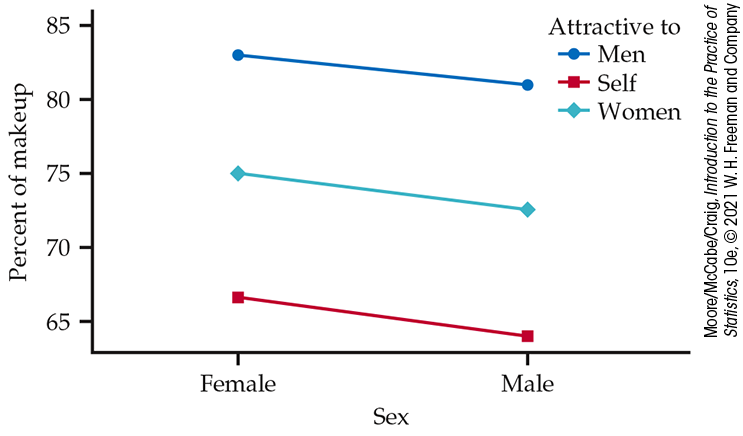
Figure 13.4 Interaction plot, Exercise 13.8.
-
-
13.9 Alternative interaction plot. In Figure 13.2 (page 659), the interaction plot involves two profiles because group size was used on the x axis. Construct the alternative interaction plot involving five profiles by using location on the x axis. Which of these two interaction plots do you prefer, and why?
-
13.10 Proposing a two-factor design. A paint supplier is interested in assessing the hardness of four brands of paint, each with and without an additive that is supposed to add durability. The supplier has a total of 40 panels that can be painted. Hardness will be measured after 180 days of weathering, using an automatic scratch hardness tester. Propose a two-factor design to use for this study, using a two-way table similar to that on page 652.
-
13.11 Compare employee training programs. A company wants to compare three different training programs for its new employees. Each of these programs takes six hours to complete. The training can be given for six hours on one day or for three hours on two consecutive days. The next 100 employees hired by the company will be the subjects for this study. After the training is completed, the employees will be asked to evaluate the effectiveness of the program through a series of questions on a seven-point scale. Propose a two-factor design to use for this study using a two-way table similar to that on page 652.