12.1 Inference for One-Way Analysis of Variance
When comparing different populations or groups, the data are subject to sampling variability. For example, we would not expect to observe exactly the same sales data if we mailed an advertising offer to different random samples of households. We also wouldn’t expect a new group of cancer patients to provide the same set of progression-free survival times.
Because of this variability, we pose the question for inference in terms of the mean response. In Section 7.2 (page 410), we met procedures for comparing the means of two populations. We now extend those methods to problems involving the means of more than two populations. Although the details differ, many of the concepts are similar to those discussed in the two-sample case.
The statistical methodology for comparing several means is analysis of variance (ANOVA). In the previous two chapters we used analysis of variance to assess the linear relationship between the subpopulation means and explanatory variables. In this section and the following one, we will examine the basic ideas and assumptions that are needed for ANOVA in this setting.
We will consider two ANOVA techniques. When there is only one way to classify the populations of interest, we use one-way ANOVA to analyze the data. We call this categorical explanatory variable a factor. For example, to compare the average tread lifetimes of six concept tires, we use one-way ANOVA with tire type as our factor. This chapter presents the details for one-way ANOVA.
In many other comparative studies, there is more than one way to classify the populations. For the tire study, the researcher team might also consider tread life under three different road temperatures. How much greater will the wear be for each concept tire at a high temperature? Are there certain types that do relatively better in a hotter environment? Analyzing the effect of tire type and temperature together requires two-way ANOVA. This technique is discussed in the next chapter.
The one-way ANOVA setting
The data for one-way ANOVA are collected just as data are collected in the two-sample case. We either draw a random sample from each population or we randomly divide subjects into different treatments. The resulting data are used to test the null hypothesis that the means are all equal.
Consider the following two examples.
Example 12.1 Does haptic feedback improve performance?
A group of technology students is interested in whether haptic feedback (forces and vibrations applied through a game controller) is helpful in navigating a simulated game environment they created. To investigate this, they randomly assign 20 participants to each of three game controller types and record the time it takes to complete a navigation mission. The controller types are (1) a standard video game controller, (2) a game controller with force feedback, and (3) a game controller with vibration feedback.
Example 12.2 Average age of coffeehouse customers.
How do five coffeehouses around campus differ in the demographics of their customers? Are certain coffeehouses more popular among graduate students? Do professors tend to favor one coffeehouse? A reporter from the student newspaper asks 50 customers of each coffeehouse to respond to a questionnaire. One variable of interest is the customer’s age.
These two examples are similar in that
- There is a single quantitative response variable measured on many units; the units are the 60 participants in the first example and the 250 customers in the second.
- The goal is to compare several populations: participants using three different game controller types in the first example and customers of the five coffeehouses in the second.
- There is a single categorical explanatory variable, or factor, that classifies these populations: controller type in the first example and coffeehouse in the second.
There is, however, an important difference. Example 12.1 describes an experiment in which each participant is randomly assigned to a type of game controller. Example 12.2 is an observational study in which customers are selected during a particular time period, and not all agree to provide data. This means that the samples in the second example are not truly SRSs. The reporter will treat them as such because she believes that the selective sampling and nonresponse are ignorable sources of bias and variability, but others may not agree. Always consider the sampling design and various sources of bias in an observational study.
In both examples, one-way ANOVA is used to compare the mean responses.
The same ANOVA methods apply to data from randomized experiments (Example 12.1) and to data from random samples (Example 12.2).
![]() However, it is important to keep in mind the data-production method
when interpreting the results. A strong case for causation is best made by a randomized
experiment.
However, it is important to keep in mind the data-production method
when interpreting the results. A strong case for causation is best made by a randomized
experiment.
Comparing means
The question we ask in one-way ANOVA is “Do all groups have the same population mean?” (We will often use the term groups for the populations to be compared in a one-way ANOVA.) To answer this question, we compare the sample means. Figure 12.1 displays the sample means for Example 12.1. It appears that a game controller with force feedback has the shortest average completion time. But is the observed difference in sample means just the result of chance variation? We should not expect sample means to be equal even if all groups have the same mean.
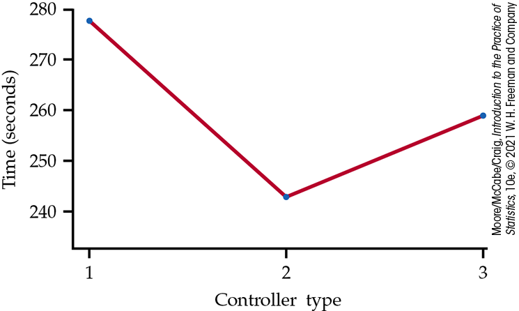
Figure 12.1 Average completion times for three different controller types, Example 12.1.
The purpose of one-way ANOVA is to assess whether the observed
differences among sample means are statistically significant.
Could variation among the three sample means this large be plausibly
due to chance, or is it strong evidence for a difference among the
group means? This question can’t be answered from the sample means
alone. Because the standard deviation of a sample mean
Side-by-side boxplots help us see the variation within the groups. Compare Figures 12.2(a) and 12.2(b). The sample medians are the same in both panels, but the large variation within the groups in Figure 12.2(a) suggests that the differences among the sample medians could be due simply to chance variation. The data in Figure 12.2(b) are much more convincing evidence that the populations differ.
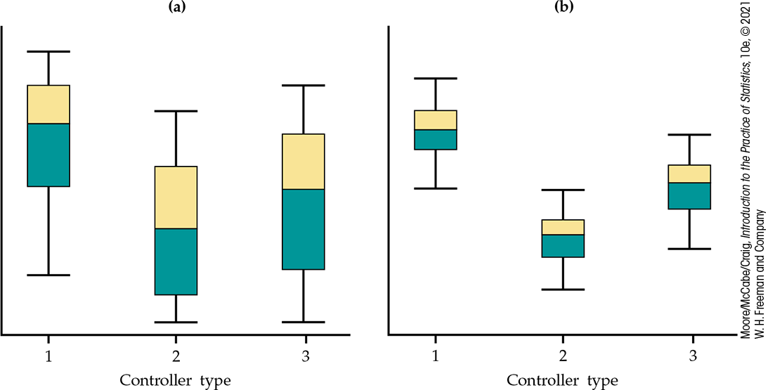
Figure 12.2(a) Side-by-side boxplots for three groups with large within-group variation. The differences among centers may be just chance variation. (b) Side-by-side boxplots for three groups with the same centers as in panel (a) but with small within-group variation. The differences among centers are more likely to be significant.
Even the boxplots omit essential information, however. To assess the observed differences, we must also know how large the samples are. Nonetheless, boxplots provide a good preliminary display of the data.
Although one-way ANOVA compares means and boxplots display medians, these two measures of center will be close together for distributions that are nearly symmetric. This is something we need to check prior to inference. If the distributions are strongly skewed, the means are not good summaries of the population centers. We may, for example, consider a transformation prior to displaying and analyzing the data.
The two-sample t statistic
Two-sample t statistics compare the means of two populations. If the two populations are assumed to have equal but unknown standard deviations and the sample sizes are both equal to n, the t statistic is
The square of this t statistic is
If we use one-way ANOVA to compare two populations, the ANOVA
F statistic is exactly equal to this
The numerator in the
The denominator measures the
within-group
variation
by
Although the general form of the one-way ANOVA F statistic is more complicated, the idea is the same. To assess whether several populations all have the same mean, we compare the variation among the means of several groups with the variation within groups. Just like with linear regression, we are comparing variation so the method is called analysis of variance.
Check-in
-
12.1 What’s wrong? In each of the following, explain what is wrong and why.
-
ANOVA tests the null hypothesis that the sample means are all equal.
-
A strong case for causation is best made by an observational study.
-
One-way ANOVA is used to test whether the population variances are the same.
-
A two-way ANOVA is used to compare the means of two populations.
-
-
12.2 Viewing side-by-side boxplots. Consider the coffeehouse setting in Example 12.2 (page 600) and assume that all the coffeehouse means are the same except for the second coffeehouse, which has a lower average age. Using Figure 12.2 as a guide, sketch possible side-by-side boxplots for the following two situations:
-
The within-group variation is small enough that ANOVA will almost surely detect that the means differ.
-
The within-group variation is so large that ANOVA likely will not detect this difference in means.
-
An overview of ANOVA
Now that we have a general idea of how one-way ANOVA works, we will explore the specifics using an example. Because the computations are more lengthy than those for the t test, we generally use computer software to perform the calculations. Automating the calculations frees us from the burden of needing to perform arithmetic and allows us to concentrate on interpretation.
Example 12.3 Task performance with background music.
![]()

The effect of music on task performance has long been of interest to researchers. The “Mozart effect” is one of the first, most well-known, and controversial explanations of music’s influence. It suggests a short-term increase of 8 to 9 points in mean spatial IQ score after listening to Mozart’s Sonata for Two Pianos (K448).2 Subsequent research has looked at replicating these results as well as looking at the effect with different types of tasks, different types of music, and different levels of volume. Findings have been mixed, with some suggesting music improved performance, others suggesting music hindered performance, and still others finding no evidence of an effect.
One experiment compared the performance of various tasks under three different types of background music conditions: silence, music with lyrics, and music conditions without lyrics.3 For our analysis, we will focus just on the mathematics task, which involved solving as many simple arithmetic problems as possible in a minute.
A total of 452 participants were recruited through Amazon Mechanical Turk (MTurk), which is a crowdsourcing marketplace. Of these, only 447 completed the mathematics task. Here is a summary of the data for the number of completed simple arithmetic problems x in a minute:
| Group | n |
|
s |
|---|---|---|---|
| Silence | 152 | 18.855 | 4.690 |
| Music without lyrics | 149 | 17.745 | 4.175 |
| Music with lyrics | 146 | 17.815 | 4.238 |
It appears that music results in a decrease in production of about one problem and that there is very little difference between the types of music. ANOVA will allow us to determine whether this observed pattern in sample means can be extended to the group means.
We should always start our ANOVA with a careful examination of the
data using graphical and numerical summaries.
![]() Complicated computations do not guarantee a valid statistical
analysis. This examination gives us an idea of what to expect from the
analysis and also enables us to check for unusual patterns in the
data. Just as with the two-sample t methods and linear
regression, outliers and extreme deviations from Normality can
invalidate the computed results.
Complicated computations do not guarantee a valid statistical
analysis. This examination gives us an idea of what to expect from the
analysis and also enables us to check for unusual patterns in the
data. Just as with the two-sample t methods and linear
regression, outliers and extreme deviations from Normality can
invalidate the computed results.
Example 12.4 A graphical summary of the data.
![]()
Let’s use the labels 1, 2, and 3 to represent silence, music without lyrics, and music with lyrics, respectively. Histograms for the three groups are given in Figure 12.3. Note that the heights of the bars are percents rather than counts. Percents are commonly used when the group sample sizes vary. Figure 12.4 gives side-by-side boxplots for these data. We see a lot of spread in the data, with the number of completed problems ranging from 6 to 31.
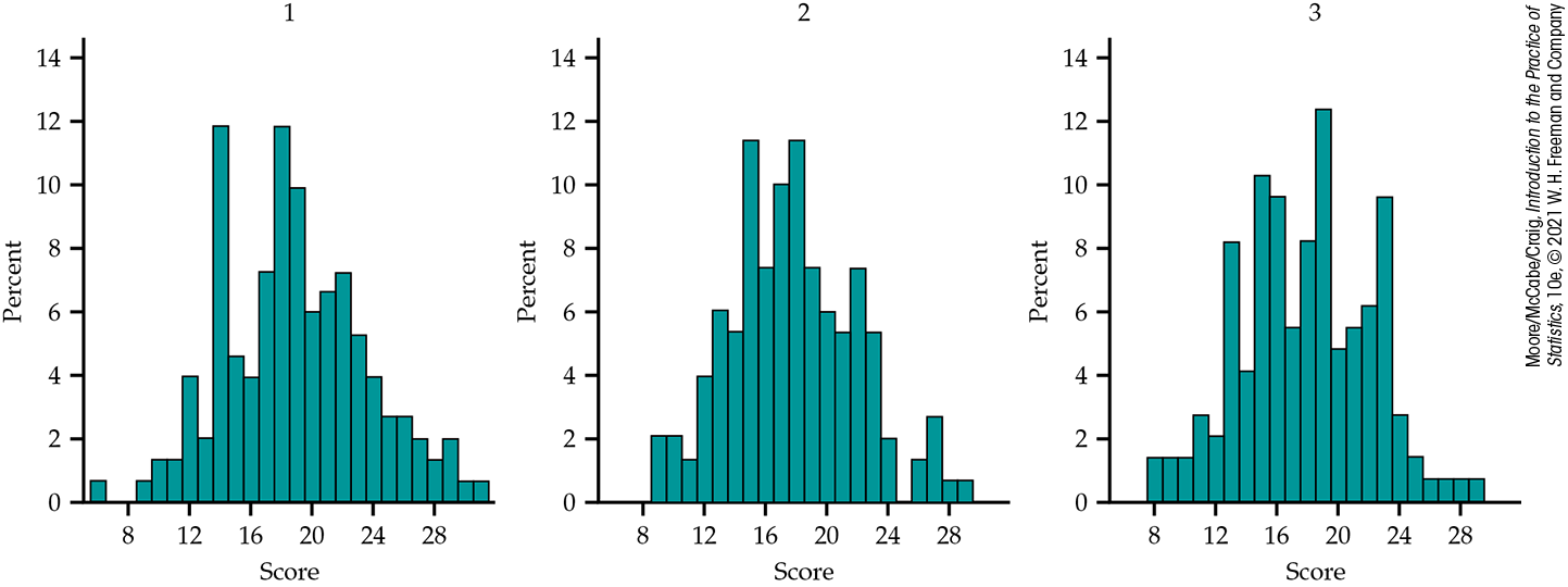
Figure 12.3 Histograms of music groups, Example 12.4.
There do not appear to be any outliers, and the distributions appear relatively symmetric. Even though the data are counts, the fact that the group sample sizes are all more than 45 suggests that we can feel confident that the sample means are approximately Normal. As with the two-sample procedures, it is important for the sample means, rather than the data, to be approximately Normal.
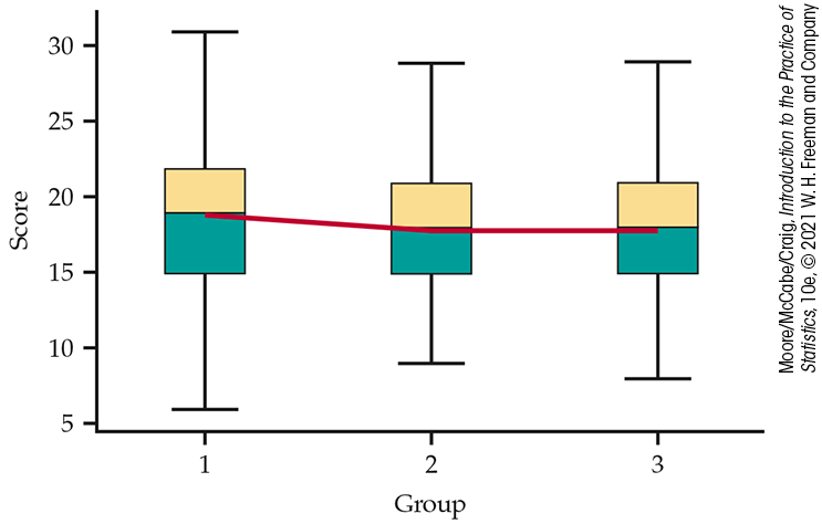
Figure 12.4 Side-by-side boxplots for the background music study, Example 12.4. The three sample means are also shown using connecting lines.
Figure 12.4 also includes the three means adjacently joined with a line. The difference in means pales in comparison to the variability within each group. This suggests that the observed pattern in the means could likely be due to chance variation.
Including the mean in a boxplot is quite common. Joining the means of side-by-side boxplots is less common, and some do not like it. It is done here to help show the differences in sample means relative to the spread in the data. Oftentimes, combined plots like this one—a combination of a mean plot (e.g., Figure 12.1) and side-by-side boxplots—can be more helpful than separate, more traditional ones. Do you think it is more helpful here?
The setting of this example is an experiment in which participants were randomly assigned to one of the three groups. Each of these groups has a mean, and our inference asks questions about these means. The participants were all recruited from MTurk and participated online. They were paid $1.00 in return for completing the study. The authors also state that they were properly motivated to take the tasks seriously using an incentive payment of $5.00 that went to the participant with the highest performance.
![]() Formulating a clear definition of the populations being compared
with ANOVA can be difficult. Often some expert judgment is required, and different consumers of
the results may have different opinions. Whether we can comfortably
generalize our conclusions of this study to the population of MTurk
workers or to the general population of adults is open to debate.
Using MTurk is quite popular because it supplies a large number of
potential participants at very low cost. The trade-off is more
difficulty in clearly defining the populations. Regardless, we are
more confident in generalizing our conclusions to similar populations
when the results are clearly significant than when the level of
significance just barely passes the standard of
Formulating a clear definition of the populations being compared
with ANOVA can be difficult. Often some expert judgment is required, and different consumers of
the results may have different opinions. Whether we can comfortably
generalize our conclusions of this study to the population of MTurk
workers or to the general population of adults is open to debate.
Using MTurk is quite popular because it supplies a large number of
potential participants at very low cost. The trade-off is more
difficulty in clearly defining the populations. Regardless, we are
more confident in generalizing our conclusions to similar populations
when the results are clearly significant than when the level of
significance just barely passes the standard of
Check-in
-
12.3 Biased results? For the study in Example 12.3, 560 MTurk workers participated in the study, but only 452 completed the study. Furthermore, the data from an additional 5 participants were not used in the analysis of the math task. The authors say that the 108 who did not complete the study either dropped out partway or encountered some technical issue, such as a bad Internet connection. The authors do not supply a reason for the additional 5 participants. Do you think this roughly 20% dropout rate biases the results of this study? Write a short paragraph explaining your answer.
-
12.4 Defining the population. For the study in Example 12.3, we are told that of the 452 participants who completed the study, 62.6% identified as male and 36.7% identified as female. In terms of ethnicity, the breakdown was as follows: 47.6% were Caucasian, 39.6% Asian/Pacific Islander, 5.5% Black/African American, and 3.3% Hispanic/Latinx. For age, the breakdown was 9.5% 18–24, 43.3% 25–30, 33.9% 31–40, 9.7% 41–50, and 3% 51–60. Do you think this sample can be considered representative of adults in the United States? Provide an explanation with your answer.
For inference, we first ask whether or not there is sufficient
evidence in the data to conclude that the corresponding group means
are not all equal. Our null hypothesis here states that the population
mean score is the same for all three groups. The alternative is that
they are not all the same.
![]() Rejecting the null hypothesis that the means are all the same is
not the same as concluding that all the means are different from one
another. The one-way ANOVA alternative hypothesis can be true in many
different ways. It could be true because all the means are different
or simply because one of them differs from the rest.
Rejecting the null hypothesis that the means are all the same is
not the same as concluding that all the means are different from one
another. The one-way ANOVA alternative hypothesis can be true in many
different ways. It could be true because all the means are different
or simply because one of them differs from the rest.
Because the one-way ANOVA alternative is a more complex situation than the two-population comparison alternative, we need to perform some further analysis if we reject the null hypothesis. This additional analysis allows us to draw conclusions about which population means differ from which others and by how much.
For the music study, the researchers hypothesize that background
music should negatively impact performance. Therefore, a reasonable
question to ask is whether the mean for the silence group is larger
than the others. When there are particular versions of the alternative
hypothesis that are of interest, we use contrasts to examine
them.
![]() Note that to use contrasts, it is necessary that the questions of
interest be formulated before examining the data. It is cheating to make up the questions after analyzing the data.
Note that to use contrasts, it is necessary that the questions of
interest be formulated before examining the data. It is cheating to make up the questions after analyzing the data.
If we have no specific relationships among the means in mind before looking at the data, we instead use a multiple-comparisons procedure to determine which pairs of population, or group, means differ significantly. We explore both contrasts and multiple comparisons in the next section.
The ANOVA model
When analyzing data, the following equation reminds us that we look for an overall pattern in the data and deviations from it:
In the regression model, the FIT was the population regression equation, and the RESIDUAL represented the deviations of the data from it. We now apply this framework to describe the statistical models used in one-way ANOVA. These models provide a convenient way to summarize the conditions that are the foundation for our analysis. They also give us the necessary notation to describe the calculations needed.
Recall the statistical model for a random sample of observations from
a single Normal population with mean
we can describe this model by saying that the
The
way of thinking. The FIT part of the model is represented by
There are two unknown parameters in this statistical model:
The model for one-way ANOVA is very similar. We take random samples
from each of I different populations. The sample size is
Note that the sample sizes
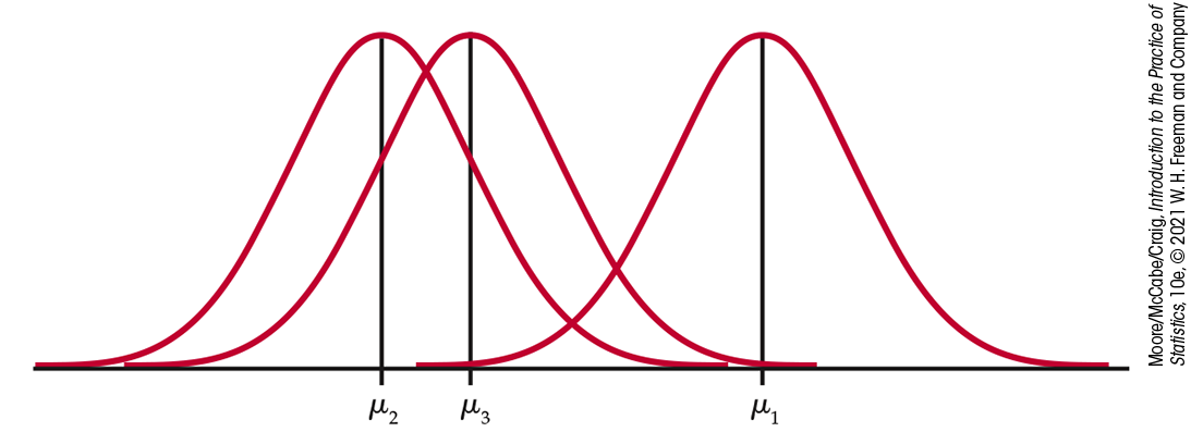
Figure 12.5 Model for one-way ANOVA with three groups. The three populations have Normal distributions with the same standard deviation.
Example 12.5 ANOVA model for the music study.
In the music study, there are three groups that we want to compare,
so
The observation
According to our model, the score for the first participant in
Condition 1 is
The ANOVA model assumes that these deviations
Check-in
-
12.5 Time to complete a navigation mission. Example 12.1 (page 600) describes a study designed to compare different controller types on the time it takes to complete a navigation mission. Write out the ANOVA model for this study. Be sure to give specific values for I and the
-
12.6 Ages of customers at different coffeehouses. In Example 12.2 (page 600), the ages of customers at different coffeehouses are compared. Write out the ANOVA model for this study. Be sure to give specific values for I and the
Estimates of population parameters
The unknown parameters in the statistical model for ANOVA are the
I population means
The residuals
In addition to the deviations being Normally distributed, the one-way
ANOVA model also states that the population standard deviations are
all equal. Before estimating
Because one-way ANOVA procedures are not extremely sensitive to unequal standard deviations, especially when the group sample sizes are similar, we do not recommend a formal test of equality of standard deviations as a preliminary to the ANOVA. Instead, we will use the following rule of thumb.
If there is evidence that we have unequal group standard deviations,
we generally try to transform the data so that they are approximately
equal. We might, for example, work with
Example 12.6 Are the standard deviations equal?
![]()
In the music study, there are
When we assume that the population standard deviations are equal, each
sample standard deviation is an estimate of
Pooling gives more weight to groups with larger sample sizes. If the
sample sizes are equal,
![]() Note that
Note that
Example 12.7 The common standard deviation estimate.
![]()
In the music study, there are
The pooled sample variance is
The pooled standard deviation is
This is our estimate of the common standard deviation
Check-in
-
12.7 Game controller types. Example 12.1 (page 600) describes a study designed to compare different controller types on the time it takes to complete a navigation mission. In Check-in question 12.5 (page 608), you described the ANOVA model for this study. The three controller types are designated 1, 2, and 3. The following table summarizes the time data:
Controller s n 1 279 78 20 2 245 68 20 3 258 80 20 -
Is it reasonable to pool the standard deviations for these data? Explain your answer.
-
For each parameter in your model from Check-in question 12.5, give the estimate.
-
-
12.8 Ages of customers at different coffeehouses. In Example 12.2 (page 600), the ages of customers at different coffeehouses are compared, and you described the ANOVA model for this study in Check-in question 12.6 (page 608). It turned out that roughly 25% of those surveyed declined to respond. Here is a summary of the ages of the customers who responded:
Store s n A 39 8 39 B 47 13 38 C 41 11 42 D 26 7 38 E 34 10 43 -
Is it reasonable to pool the standard deviations for these data? Explain your answer.
-
For each parameter in your model from Check-in question 12.6, give the estimate.
-
Testing hypotheses in one-way ANOVA
Comparison of several means is accomplished by using an F statistic to compare the variation among groups with the variation within groups. We now show how the F statistic expresses this comparison. Calculations are organized in an ANOVA table, which contains numerical measures of the variation among groups and within groups.
First, we must specify our hypotheses for one-way ANOVA. As before, I represents the number of populations to be compared.
Before proceeding to inference, we should verify the conditions necessary for the one-way ANOVA results to be trusted. There is no point in doing this analysis if the data do not, at least approximately, meet these conditions.
Example 12.8 Verifying the conditions for ANOVA.
![]()
We’ve discussed each of these conditions already. Here is a summary of our assessments for the music study.
SRSs. This is an experiment in which participants were randomly assigned to groups. We clearly have SRSs, but defining the population from which we obtained the participants is challenging. They were all recruited from MTurk and were paid to participate. Can we act as if they were randomly chosen from the general population of adults? People may disagree on the answer.
Normality. Are the number of problems completed Normally distributed in each group? We’ve already argued they are not Normally distributed, but because inference is based on the sample means and we have very large sample sizes, we are not concerned about violating this condition. The exception would be if there were outliers or extreme skewness. Figure 12.6 displays the Normal quantile plots for each of the three groups. There are no outliers and no strong departures from Normality.
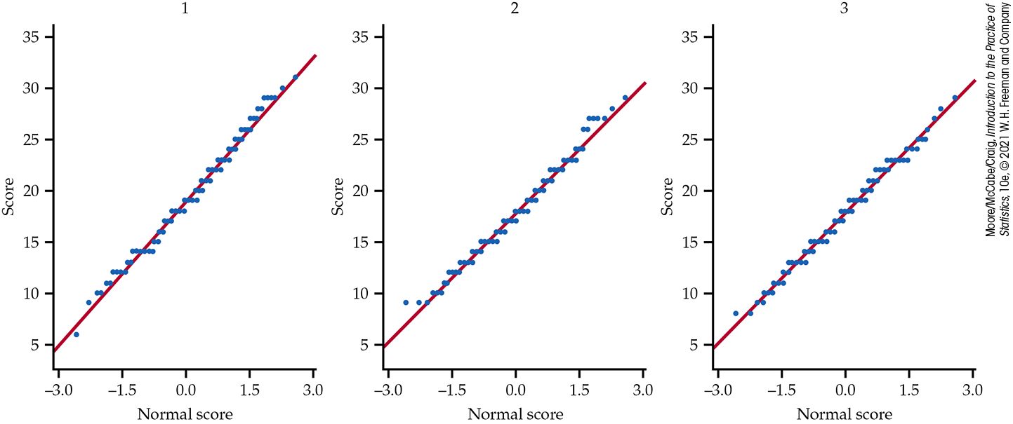
Figure 12.6 Normal quantile plots of the number of problems completed for the three background music groups, Example 12.8.
Common standard deviation. Are the population standard deviations equal? Because the largest sample standard deviation is not more than twice the smallest sample standard deviation, we can proceed, assuming that the population standard deviations are equal.
Check-in
-
12.9 An alternative Normality check. Figure 12.6 displays Normal quantile plots for each of the three background music groups. An alternative procedure to check Normality is to make one Normal quantile plot using the residuals

-
12.10 An alternative Normality check (continued). Refer to the previous Check-in question. Describe the benefits and drawbacks of checking Normality using all the residuals together versus looking at each group sample separately. Which approach do you prefer and why?
Having determined that the data approximately satisfy these three conditions, we proceed with inference.
Example 12.9 Reading software output.
![]()
Figure 12.7
shows descriptive statistics generated by JMP for the music study.
Summaries for each background music group are given on the first
three lines. In addition to the sample size, the mean, and the
standard deviation, this output also gives the minimum and maximum
observed values and the standard error of the mean of each group.
The three sample means
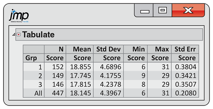
Figure 12.7 Descriptive statistics for the music study, Example 12.9.
![]()
The output gives the estimates of the standard deviations,
Some software packages report
![]() Note that
Note that
Example 12.10 Reading software output (continued).
![]()
Output for the one-way ANOVA of the music study is given in
Figure 12.8. We will discuss the construction of this output next. For now, we
observe that the results of our significance test are given in the
last two columns of the “Analysis of Variance” output. The null
hypothesis that the three group means are the same is tested by the
statistic
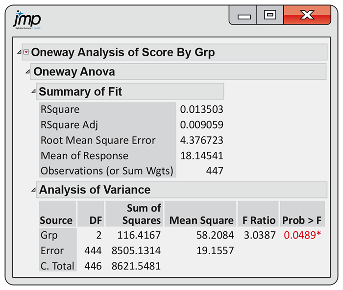
Figure 12.8 JMP analysis of variance output for the music study, Example 12.10.
![]()
The ANOVA table
For one-way ANOVA, the model is
Much as with linear regression, we can think of the information in the one-way ANOVA table in terms of our
view of statistical models. It summarizes the separation of the total variation and degrees of freedom in the data into two parts: the part due to the fit and the remainder, which we call residual.
Example 12.11 ANOVA table for the music study.
The JMP output in Figure 12.8 gives the sources of variation in the first column. Here, FIT is called Grp, the name of the factor, RESIDUAL is called Error, and DATA is the last entry, C. Total. Different software packages use different names for these sources of variation, but the basic concept is common to all. Other names for FIT may be “Between Groups” or “Model.” Another name for RESIDUAL is “Within Groups.”
The Grp row in the table gives information related to the variation among groups—in particular, their means. In expressing a general one-way ANOVA table, we will use the generic label “Groups.” The Error row in the table gives information related to the variation within groups. Although the term “Error” is frequently used for this source of variation, it is most appropriate for experiments in the physical sciences where the observations within a group differ because of measurement error. In business and the biological and social sciences, the within-group variation is often due to the fact that not all firms or plants or people are the same. This sort of variation is not due to errors and is better described as “residual” or “within-group” variation. Nevertheless, we will use the generic label “Error” for this source of variation in the general one-way ANOVA table.
Finally, the C. Total row in the one-way ANOVA table corresponds to the DATA term in our view of statistical models. So, for one-way analysis of variance,
translates into
The second and third columns in the software output given in
Figure 12.8 are labeled “DF”
and “Sum of Squares.” As you might expect, each sum of squares is a
sum of squared deviations. We use SSG, SSE, and SST for the entries in
this column, corresponding to groups, error, and total. Each sum of
squares measures a different type of variation. SST measures variation
of the data around the overall mean,
Associated with each sum of squares is a quantity called the degrees
of freedom, labeled “DF.” Because SST measures the variation of all
N observations around the overall mean, its degrees of freedom
are
Example 12.12 ANOVA table for the music study (continued).
The “Sum of Squares” column in Figure 12.8 gives the values for the three sums of squares. They are
As we’ve seen before, total variation is always equal to the
among-group variation plus the within-group variation. That is,
In this study, we have
These are the entries in the “DF” column of
Figure 12.8. Again, the
degrees of freedom add in the same way—that is,
In this music study, most of the variation is coming from within groups. For a one-way analysis of variance, we define the coefficient of determination as
The coefficient of determination plays the same role as the squared
multiple correlation
Example 12.13 Coefficient of determination for the music study.
The software-generated ANOVA table for the music study is given in
Figure 12.8 (page 618). From that display, we see that
Only 1.4% of the variation in the number of completed math problems is explained by the different background music levels. The other 98.6% of the variation is due to participant-to-participant variation within each of the groups. We can see this in the boxplots of Figure 12.4 (page 604). Each of the groups has a large amount of variation, and there is a substantial amount of overlap in their distributions.
To assess whether the observed differences in sample means are statistically significant, some additional calculations are needed. For each source of variation, the mean square is the sum of squares divided by the degrees of freedom. You can verify this by doing the divisions for the values given on the output in Figure 12.8. We compare these mean squares to test whether the population means are all the same.
We can use the mean square for error to find
In other words, the mean square for error is an estimate of the
within-group variance,
Example 12.14 The pooled
estimate for
σ
From the JMP output in
Figure 12.8, we see that
the MSE is reported as 19.1557. The pooled estimate of
This estimate is equal to our calculations of
The F test
If
When
![]() When determining the P-value, remember that the F test is always
one-sided because any differences among the group means tend to make
F large.
When determining the P-value, remember that the F test is always
one-sided because any differences among the group means tend to make
F large.
Example 12.15 The ANOVA F test for the music study.
In the music study, we found
If only the F statistic were provided, we’d need to use
software or Table E to approximate the P-value. To get the
P-value using Excel, we would
|
|
|
|---|---|
| p | Critical value |
| 0.100 | 2.33 |
| 0.050 | 3.04 |
| 0.025 | 3.76 |
| 0.010 | 4.71 |
| 0.001 | 7.15 |
Even though the group means explain only 1.4% of the total
variability, the F test is statistically significant at the
![]() A significant F test does not necessarily mean that the
distributions of values are far apart.
A significant F test does not necessarily mean that the
distributions of values are far apart.
![]() Using the One-Way ANOVA applet is an excellent way to see how
the value of the F statistic and the P-value depend upon
the variability of the data within the groups, the sample sizes, and
the differences between the means. See
Exercises 12.44, 12.45, and
12.46 (page 642) for use of this applet.
Using the One-Way ANOVA applet is an excellent way to see how
the value of the F statistic and the P-value depend upon
the variability of the data within the groups, the sample sizes, and
the differences between the means. See
Exercises 12.44, 12.45, and
12.46 (page 642) for use of this applet.
The one-way ANOVA F test shares the robustness of the two-sample t test. It is relatively insensitive to moderate non-Normality and unequal variances, especially when the sample sizes are similar. The constant variance assumption is more important when we compare means using contrasts and multiple comparisons, which are additional analyses that are performed after the ANOVA F test. We discuss these analyses in the next section.
The following display shows the general form of a one-way ANOVA table with the F statistic. The formulas in the sum of squares column can be used for calculations in small problems. There are other formulas that are more efficient for hand or calculator use, but ANOVA calculations are usually done by computer software.
| Source | Degrees of freedom | Sum of squares | Mean square | F |
|---|---|---|---|---|
| Groups |
|
|
SSG/DFG | MSG/MSE |
| Error |
|
|
SSE/DFE | |
| Total |
|
|
Check-in
-
12.11 What’s wrong? In each of the following, identify what is wrong and then either explain why it is wrong or change the wording of the statement to make it true.
-
Within-group variation is the variation in the data due to the differences in the sample means.
-
The mean squares in an ANOVA table will add—that is,
-
The pooled estimate
-
A very small P-value implies that the group distributions of responses are far apart.
-
-
12.12 Determining the critical value of F. For each of the following situations, state how large the F statistic needs to be for rejection of the null hypothesis at the 0.05 level.
-
Compare three groups with four observations per group.
-
Compare three groups with five observations per group.
-
Compare four groups with five observations per group.
-
Summarize what you have learned about F distributions from this exercise.
-
Software
![]()
We used JMP to illustrate the analysis of the music study. Other statistical software gives similar output, and you should be able to read it without any difficulty. Here’s an example on which to practice this skill.
Example 12.16 Do eyes affect ad response?
![]()

Research from a variety of fields has found significant effects of eye gaze and eye color on emotions and perceptions such as arousal, attractiveness, and honesty. These findings suggest that a model’s eyes may play a role in a viewer’s response to an advertisement.
In one study, students in marketing and management classes of a southern, predominantly Hispanic, university were each presented with one of four portfolios.5 Each portfolio contained a target ad for a fictional product, Sparkle Toothpaste. Students were asked to view the ad and then respond to questions concerning their attitudes and emotions about the ad and product. All questions were from advertising-effects questionnaires previously used in the literature. Each response was on a seven-point scale.
Although the researchers investigated nine attitudes and emotions, we will focus on the viewer’s “attitudes toward the brand.” This response was obtained by averaging 10 survey questions.
The target ads were created using two digital photographs of a model. In one picture, the model is looking directly at the camera so the eyes can be seen. This picture was used in three target ads. The only difference was the model’s eyes, which were made to be either brown, blue, or green. In the second picture, the model is in virtually the same pose but looking downward so the eyes are not visible. A total of 222 surveys were used for analysis. Outputs from Excel, JMP, and Minitab are given in Figure 12.9.
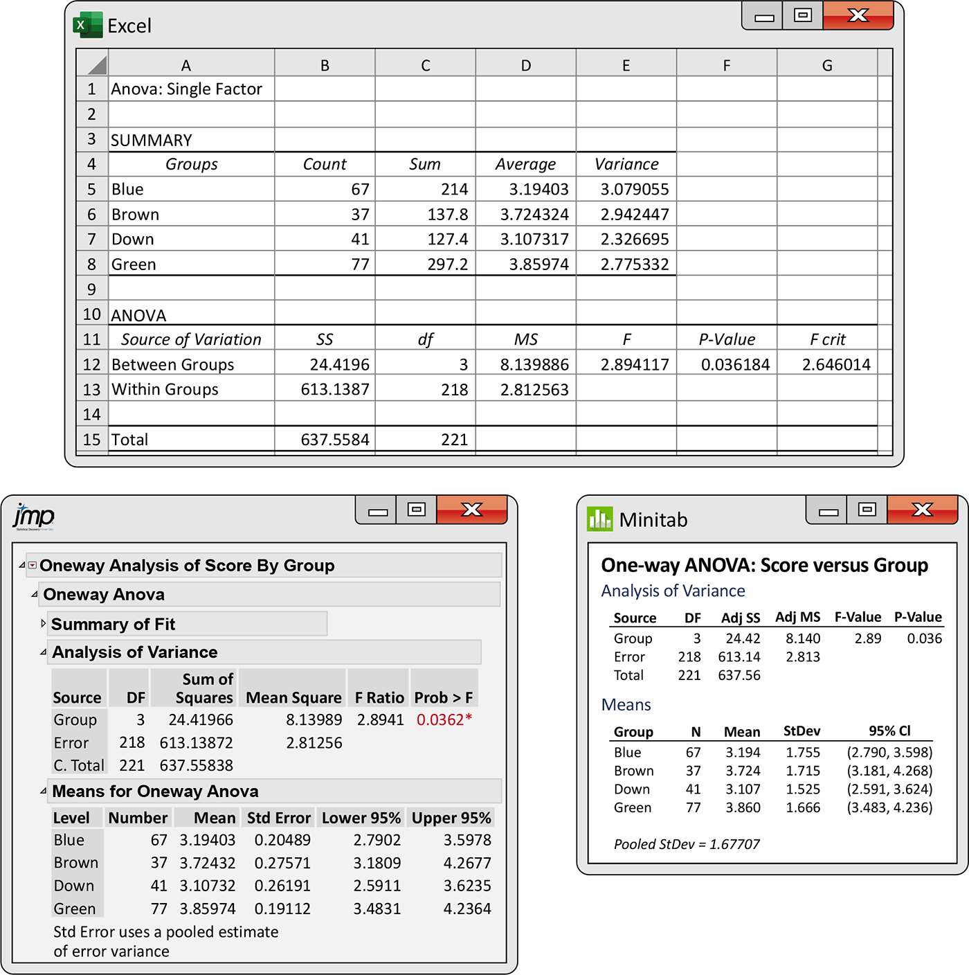
Figure 12.9 Excel, JMP, and Minitab outputs for the advertising study, Example 12.16.
There is evidence at the 5% significance level to reject the null
hypothesis that the four groups have equal means
This test uses a more robust measure of deviation, replacing the mean with the median and replacing squaring with the absolute value. Also, the creation of the transformed response variable is straightforward, so this test can be performed regardless of whether your software specifically has it.
Example 12.17 Are the standard deviations equal?
![]()
Figure 12.10
shows output of the modified Levene’s test for the advertisement
study. In JMP, the test is called Brown–Forsythe. The P-value
is 0.6775, which is much larger than
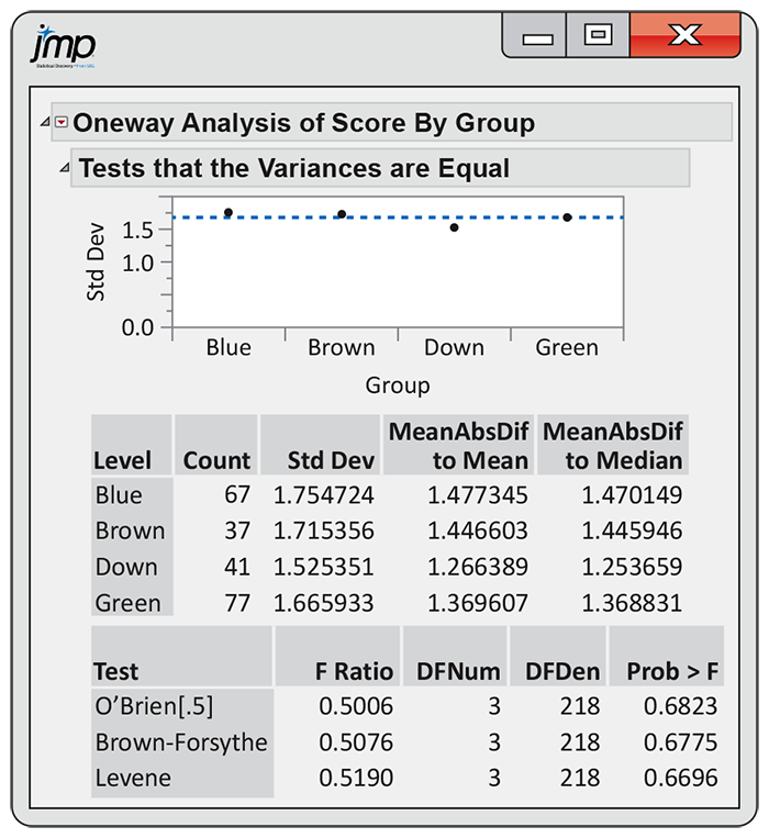
Figure 12.10 JMP output for the test that the variances are equal, Example 12.17.
Remember that our rule of thumb (page 608) is used to assess whether different standard deviations will
impact the ANOVA results.
![]() It’s not a formal test that the standard deviations are equal. There will be times when the rule and formal test do not agree.
It’s not a formal test that the standard deviations are equal. There will be times when the rule and formal test do not agree.
Section 12.1 SUMMARY
-
One-way analysis of variance (ANOVA) is used to compare several population means based on independent SRSs from each population. The populations are assumed to be Normal, with possibly different means and the same standard deviation.
-
To do an analysis of variance, first examine the data. The model conditions only need to be approximately met in order to obtain valid results. Side-by-side boxplots give an overview of the data. Normal quantile plots and histograms (either for each group separately or for the residuals) allow you to detect outliers or extreme deviations from Normality.
-
In addition to Normality, the ANOVA model assumes equal population standard deviations. Compute the ratio of the largest to the smallest sample standard deviation. If this ratio is less than 2 and the Normality condition is reasonable, ANOVA can be performed.
-
If the data do not support equal standard deviations, consider transforming the response variable. This often makes the group standard deviations more nearly equal and makes the group distributions more Normal. If the standard deviations cannot be made similar by a transformation, inference requires different methods such as nonparametric methods or the bootstrap.
-
ANOVA is based on separating the total variation observed in the data into two parts: between-group variation and within-group variation. If the variation among groups is large relative to the variation within groups, we have evidence against the null hypothesis.
-
The one-way ANOVA table organizes the ANOVA calculations. Degrees of freedom, sums of squares, and mean squares appear in the table. The F statistic and its P-value are used to test the null hypothesis.
-
The coefficient of determination
is the proportion of variation explained by the group means
-
The null hypothesis of the one-way ANOVA F test is that the group means are all equal. The alternative hypothesis is true if there are any differences among the group means.
-
The ANOVA F test shares the robustness of the two-sample t test. It is relatively insensitive to moderate non-Normality and unequal variances, especially when the sample sizes are similar.
Section 12.1 EXERCISES
-
12.1 A one-way ANOVA example. A study compared four groups with five observations per group. An F statistic of 3.78 was reported.
-
Give the degrees of freedom for this statistic and the entries from Table E that correspond to the F distribution under the null hypothesis.
-
Sketch a picture of this F distribution with the information from Table E included.
-
Given the reported F statistic, how would you report the P-value?
-
If
-
-
12.2 Visualizing the ANOVA model. For each of the following settings, draw a picture of the ANOVA model similar to Figure 12.5 (page 607). To sketch the Normal curves, you may want to review the 68–95–99.7 rule on page 51.
-
-
12.3 Visualizing the ANOVA model (continued). Refer to the previous exercise. If SRSs of size
-
12.4 Calculating the ANOVA F test P-value. For each of the following situations, find the degrees of freedom for the F statistic and then use Table E (or software) to approximate (obtain) the P-value.
-
Five groups are being compared, with 5 observations per group. The value of the F statistic is 3.47.
-
Four groups are being compared, with 11 observations per group. The value of the F statistic is 4.28.
-
Five groups are being compared, with 65 total observations. The value of the F statistic is 2.97.
-
-
12.5 Calculating the ANOVA F test P-value (continued). For each of the following situations, find the F statistic and the degrees of freedom. Then draw a sketch of the distribution under the null hypothesis and shade in the portion corresponding to the P-value. State how you would report the P-value.
-
Compare 3 groups with 21 observations per group,
-
Compare 8 groups with 6 observations per group,
-
-
12.6 Calculating the pooled standard deviation. An experiment was run to compare three groups. The sample sizes were 32, 27, and 98, and the corresponding estimated standard deviations were 2.2, 2.4, and 4.3.
-
Is it reasonable to use the assumption of equal standard deviations when we analyze these data? Give a reason for your answer.
-
Give the values of the variances for the three groups.
Find the pooled variance.
-
What is the value of the pooled standard deviation?
-
Explain why your answer in part (d) is much closer to the standard deviation for the third group than to either of the other two standard deviations.
-
-
12.7 Describing the ANOVA model. For each of the following situations, identify the response variable and the populations to be compared and give I,
-
A poultry farmer is interested in reducing the cholesterol level in his marketable eggs. He wants to compare two different cholesterol-lowering drugs added to the hens’ standard diet as well as an all-vegetarian diet. He assigns 25 of his hens to each of the three treatments.
-
A researcher is interested in students’ opinions regarding an additional annual fee to support non-income-producing varsity sports. Students were asked to rate their acceptance of this fee on a seven-point scale. The researcher received 94 responses, of which 31 were from students who attend varsity football or basketball games only, 18 were from students who also attend other varsity competitions, and 45 were from students who did not attend any varsity games.
-
A professor wants to evaluate the effectiveness of his teaching assistants. In one class period, the 42 students were randomly divided into three equal-sized groups, and each group was taught power calculations from one of the assistants. At the beginning of the next class, each student took a quiz on power calculations, and these scores were compared.
-
-
12.8 Describing the ANOVA model (continued). For each of the following situations, identify the response variable and the populations to be compared and give I,
-
A developer of a virtual-reality (VR) teaching tool for the deaf wanted to compare the effectiveness of different navigation methods. A total of 40 children were available for the experiment, and equal numbers of children were randomly assigned to use a joystick, wand, dancemat, or gesture-based pinch gloves. The time (in seconds) to complete a designed VR path was recorded for each child.
-
To study the effects of pesticides on birds, an experimenter randomly (and equally) allocated 65 chicks to five diets (a control and four other diets, each with a different pesticide included). After a month, the calcium content (milligrams) in a 1-centimeter length of bone from each chick was measured.
-
A university sandwich shop wants to compare the effects of providing free food with a sandwich order on sales. The experiment will be conducted from 11:00 a.m. to 2:00 p.m. for the next 20 weekdays. On each day, customers will be offered one of the following: a free drink, free chips, a free cookie, or nothing. Each option will be offered five times.
-
-
12.9 Determining the degrees of freedom. Refer to Exercise 12.7. For each situation, give the following:
-
Degrees of freedom for groups, error and total sums of squares.
Null and alternative hypotheses.
-
Numerator and denominator degrees of freedom for the F statistic.
-
-
12.10 Determining the degrees of freedom (continued). Refer to Exercise 12.8. For each situation, give the following:
-
Degrees of freedom for groups, error and total sums of squares.
Null and alternative hypotheses.
-
Numerator and denominator degrees of freedom for the F statistic.
-
-
12.11 Data collection and the interpretation of results. Refer to Exercise 12.7. For each situation, discuss the method of obtaining the data and how it will affect the extent to which the results can be generalized.
-
12.12 Data collection (continued). Refer to Exercise 12.8. For each situation, discuss the method of obtaining the data and how it will affect the extent to which the results can be generalized.
-
12.13 Effects of music on imagery training. Music that matches a sports activity’s requirements has been shown to enhance sports performance. Very little, however, is known about the effects of music on imagery in the context of sports performance. In one study, 63 novice dart throwers were randomly assigned equally to three groups.7 During each of 12 dart-throwing imagery sessions, one group listened to unfamiliar relaxing music (URM), another listened to unfamiliar arousing music (UAM), and the other listened to no music (NM). Dart-throwing performance was assessed before and after the imagery sessions using a 40-dart distance score. (Darts closer to the center of the board were given a higher score.) Here are the results for the gain in score
Group s URM 37.24 5.66 UAM 17.57 5.30 NM 13.19 6.14 -
Is it reasonable to assume the variance is the same across groups? Explain your answer.
Compute the estimated common standard deviation.
-
Plot the means versus the imagery group. Do there appear to be differences in the average gain in performance? Use the estimated common standard deviation to explain your answer.
-
-
12.14 Effects of music on imagery training (continued). Refer to the previous exercise.
-
What are the numerator and denominator degrees of freedom for this study’s ANOVA F test?
-
For this study,
-
Using Table E or software, what is the P-value for this study? What are your conclusions?
-
-
12.15 The effects of two stimulant drugs. An experimenter was interested in investigating the effects of two stimulant drugs (labeled A and B). She divided 25 rats equally into five groups (placebo, Drug A low, Drug A high, Drug B low, and Drug B high) and, 20 minutes after injection of the drug, recorded each rat’s activity level (higher score is more active). The following table summarizes the results:
Treatment Placebo 11.80 17.20 Low A 15.25 13.10 High A 18.55 10.25 Low B 16.15 7.75 High B 17.10 12.50 -
Plot the means versus the type of treatment. Does there appear to be a difference in the activity level? Explain.
-
Is it reasonable to assume that the variances are equal? Explain your answer and, if reasonable, compute
-
Give the degrees of freedom for the F statistic.
-
The F statistic is 2.64. Find the associated P-value and state your conclusions.
-
-
12.16 Perceptions of social media. It is estimated that more than 90% of North American students use social media. This has prompted much research on the mental health impacts of these technologies. In one study, researchers investigated how mental health workers perceive the association between social media and mental disorders. A sample of psychiatrists from Canada completed a questionnaire, from which a perception score was obtained (a higher score indicating a stronger perceived association). The following ANOVA table summarizes a comparison of these scores across three age groups (generations):
Source DF SS MS F Age 2 137.78 68.89 0.45 Error 45 6899.54 153.32 Total 47 7037.32 -
How many psychiatrists completed the questionnaire?
What is the estimated common standard deviation?
-
What is the P-value? Make sure to specify the degrees of freedom of the F statistic.
-
State your conclusion using the P-value from part (c) and a 5% significance level.
-
-
12.17 Pain tolerance among sports teams. Many have argued that sports such as football require the ability to withstand pain from injury for extended periods of time. To see if there is greater pain tolerance among certain sports teams, a group of researchers assessed 183 male Division II athletes from five sports.8 Each athlete was asked to put his dominant hand and forearm in a 3°C water bath and keep it in there until the pain became intolerable. The total amount of time (in seconds) that each athlete maintained his hand and forearm in the bath was recorded. Following this procedure, each athlete completed a series of surveys on aggression and competitiveness. In their report, the researchers state:
A univariate between subjects (sports team) ANOVA was performed on the total amount of time athletes were able to keep their hand and forearm in the water bath, and found it to be statistically significant,
Further analysis revealed that the lacrosse and soccer players tolerated the pain for a significantly longer period of time and swimmers tolerated the pain for a significantly shorter period of time than athletes from the other teams.
-
Based on the description of the experiment, what should the degrees of freedom be for this analysis?
-
Assuming that the degrees of freedom reported are correct, data from how many athletes were used in this analysis?
-
The researchers do not comment on the missing data in their report. List two reasons these data may not have been used and, for each, explain how the omission could impact or bias the results.
-
-
 12.18 Constructing an ANOVA table. Refer to
Check-in question 12.5
(page 608). Using the
table of group means and standard deviations, construct an ANOVA
table similar to that on
page 543.
Based on the F statistic and degrees of freedom, compute
the P-value. What do you conclude?
12.18 Constructing an ANOVA table. Refer to
Check-in question 12.5
(page 608). Using the
table of group means and standard deviations, construct an ANOVA
table similar to that on
page 543.
Based on the F statistic and degrees of freedom, compute
the P-value. What do you conclude?
-
12.19 The effect of extremely low-frequency electromagnetic fields. The use of electronic devices, such as smartphones, is now part of everyday life. These devices increase our exposure to extremely low-frequency electromagnetic fields (ELF-EMF). A study involving rats was run to study long-term exposure to ELF-EMF. For one analysis, they compared the time spent in a target quadrant that the rats were taught to go to prior to different levels of extended ELF-EMF exposure.9 There were 12 rats per level of exposure. The following ANOVA table partially summarizes the results:
Source DF SS MS F ELF-EMF 4 662.86 5.70 Error Total Fill in the missing entries in the ANOVA table.
-
Test the null hypothesis that there is no difference in the average time spent at the target site across exposure levels.
-
What is the estimate of