15.3 The Kruskal-Wallis Test*
![]()
We have now considered alternatives to the two-sample t and the matched pairs tests for comparing the magnitude of responses to two treatments. To compare more than two treatments, we use one-way analysis of variance (ANOVA) if we can assume that the population standard deviations are approximately equal and the sample means are approximately Normal. What can we do when these distribution conditions are not satisfied?
Example 15.21 Task performance with background music.
![]()
Example 12.3 (page 603) describes an experiment designed to compare the performance of various tasks under three different types of background music: silence, music with lyrics, and music without lyrics. In that example and several that follow, a one-way ANOVA was used to compare the mean scores for the three conditions on a mathematics task, which involved solving as many simple arithmetic problems as possible in a minute. Data were collected from 447 participants who were recruited through Amazon Mechanical MUSIC Turk (MTurk). To illustrate the nonparametric version of one-way ANOVA known as the Kruskal-Wallis test, we will use five observations from each of the three conditions. Here are these math scores:
| Condition | Score | Condition | Score | Condition | Score |
|---|---|---|---|---|---|
| Silence | 17 | Without lyrics | 18 | With lyrics | 23 |
| Silence | 17 | Without lyrics | 11 | With lyrics | 18 |
| Silence | 20 | Without lyrics | 10 | With lyrics | 15 |
| Silence | 12 | Without lyrics | 15 | With lyrics | 19 |
| Silence | 22 | Without lyrics | 22 | With lyrics | 16 |
Hypotheses and assumptions
The ANOVA F test concerns the I means of the study populations. The ANOVA hypotheses are
The data of the study are considered to be I independent random samples, one from each of the populations. In Example 15.21, the random samples are the same size,
The Kruskal-Wallis test is a rank test that can replace the one-way ANOVA F test. The assumption about data production (independent random samples from each population) remains important, but we can relax the assumptions of Normality and equal standard deviations. We assume only that the response variable Y has a continuous distribution in each population. The hypotheses are
If all the population distributions have the same shape, these hypotheses take a simpler form. The null hypothesis is that all I distributions have the same median. The alternative hypothesis is that not all medians are equal.
Example 15.22 Hypotheses for performance and background music.
For our task performance and background music example, let’s assume that the three distributions have the same shape. Then our hypotheses are
The Kruskal-Wallis test
Recall the analysis of variance idea: The ANOVA F test rejects the null hypothesis that the mean responses are equal in all groups if the group-to-group variation of the observations is large. The idea behind the Kruskal-Wallis test is similar. We replace the observations by their ranks and reject the null hypothesis if the group-to-group variation of the ranks is large.
We now see that, like the Wilcoxon rank sum statistic, the Kruskal-Wallis statistic is based on the sums of the ranks for the groups we are comparing. The more different these sums are, the stronger the evidence that responses are systematically larger in some groups than in others.
The exact distribution of the Kruskal-Wallis statistic H under the null hypothesis depends on all the sample sizes
Example 15.23 Perform the significance test.
![]()
In Example 15.21, there are
| Score | 10 | 11 | 12 | 15 | 15 | 16 | 17 | 17 |
| Rank | 1 | 2 | 3 | 4.5 | 4.5 | 6 | 7.5 | 7.5 |
| Group | WO | WO | S | WO | W | W | S | S |
| Score | 18 | 18 | 19 | 20 | 22 | 22 | 23 | |
| Rank | 9.5 | 9.5 | 11 | 12 | 13.5 | 13.5 | 15 | |
| Group | WO | W | W | S | S | WO | W |
The ranks for each of the three conditions are
| Conditions | Ranks | Rank sums | ||||
|---|---|---|---|---|---|---|
| Silent | 3.0 | 7.5 | 7.5 | 12.0 | 13.5 | 43.5 |
| Without lyrics | 1.0 | 2.0 | 4.5 | 9.5 | 13.5 | 30.5 |
| With lyrics | 4.5 | 6.0 | 9.5 | 11.0 | 15.0 | 46.0 |
The Kruskal-Wallis statistic is, therefore,
Using Excel, the exact P-value is = CHISQ.DIST.RT
Software uses slightly different calculations related to the treatment of ties. JMP gives
In Example 15.23, we concluded that the data did not provide evidence in support of the idea that background music influences the scores on a mathematics task. Here is an example of a study where the analysis does provide evidence for us to reject the null hypotheses. In this situation, we will include a multiple comparisons method to determine which pairs of levels of the factor differ significantly.
Example 15.24 Organic foods and morals?
![]()
Organic foods are often marketed with moral terms such as “honesty” and “purity. ” Is this just a marketing strategy, or is there a conceptual link between organic food and morality? In one experiment, 62 undergraduates were randomly assigned to one of three food conditions (organic, comfort, and control).14 First, each participant was given a packet of four food types from the assigned condition and told to rate the desirability of each food on a seven-point scale. Then, each was presented with a list of six moral transgressions and asked to rate each on a seven-point scale ranging from
Exercises 12.37–12-39 (page 640) lead you through the steps required to analyze these data using a one-way ANOVA. Note that the data are discrete, with possible values of 1 through 7, and the response variable is the average of the scores for six moral transgressions. We expect that our results should be reasonable because the sample sizes are large enough for us to expect that the sample means are approximately Normal. Let’s check the results using the Kruskal-Wallis test.
Example 15.25 Kruskal-Wallis test for organic foods and morals.
The output from JMP is given in Figure 15.10. This software uses a chi-square approximation to test the null hypothesis. We reject the null hypothesis
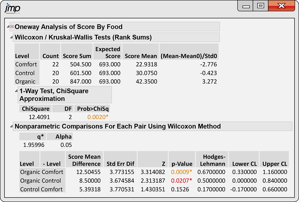
Figure 15.10 JMP output for the Kruskal-Wallis test applied to the organic food data, Example 15.25.
Section 15.3 SUMMARY
- The Kruskal-Wallis test compares several populations on the basis of independent random samples from each population. This is the one-way ANOVA setting.
- The null hypothesis for the Kruskal-Wallis test is that the distribution of the response variable is the same in all the populations. The alternative hypothesis is that responses are systematically larger in some populations than in others.
- The Kruskal-Wallis statistic H is a comparison of the sums of the ranks for the several samples.
- When the sample sizes are large and the null hypothesis is true, H for comparing I populations has approximately the chi-square distribution with
Section 15.3 EXERCISES
15.26 Do isoflavones increase bone mineral density? In Exercise 12.59 (page 645) you investigated the effects of isoflavones from kudzu on bone mineral density (BMD). The experiment randomized rats to three diets: control, low isoflavones, and high isoflavones. Here are the data:

Treatment BMD Control 0.228 0.207 0.234 0.220 0.217 0.228 0.209 0.221 0.204 0.220 0.203 0.219 0.218 0.245 0.210 Low dose 0.211 0.220 0.211 0.233 0.219 0.233 0.226 0.228 0.216 0.225 0.200 0.208 0.198 0.208 0.203 High dose 0.250 0.237 0.217 0.206 0.247 0.228 0.245 0.232 0.267 0.261 0.221 0.219 0.232 0.209 0.255 Use the Kruskal-Wallis test to compare the three diets.
How do these results compare with what you find using the ANOVA F test?
15.27 Number of Facebook friends. An experiment was run to examine the relationship between the number of Facebook friends and the user’s perceived social attractiveness.15 A total of 134 undergraduate participants were randomly assigned to observe one of five Facebook profiles. Everything about the profile was the same except the number of friends, which appeared on the profile as 102, 302, 502, 702, or 902. After viewing the profile, each participant was asked to fill out a questionnaire on the physical and social attractiveness of the profile user. Each attractiveness score is an average of several seven-point questionnaire items, ranging from 1 (strongly disagree) to 7 (strongly agree). Describe the setting for this problem. Include the number of groups to be compared, assumptions about independence, and the distribution of the attractiveness scores.

15.28 Vitamins in bread. Does bread lose its vitamins when stored? Here are data on the vitamin C content (milligrams per 100 grams of flour) in bread baked from the same recipe and stored for one, three, five, or seven days.16 The 10 observations are from 10 different loaves of bread.

Condition Vitamin C (mg/100 g) Immediately after baking 47.62 49.79 One day after baking 40.45 43.46 Three days after baking 21.25 22.34 Five days after baking 13.18 11.65 Seven days after baking 8.51 8.13 The loss of vitamin C over time is clear, but with only two loaves of bread for each storage time, we wonder if the differences among the groups are significant.
Use the Kruskal-Wallis test to assess significance and then write a brief summary of what the data show.
Because there are only two observations per group, we suspect that the common chi-square approximation to the distribution of the Kruskal-Wallis statistic may not be accurate. The exact P-value (from SAS software) is
15.29 What are the hypotheses? Refer to Exercise 15.27. What are the null hypothesis and the alternative hypothesis? Explain why a nonparametric procedure would be appropriate in this setting.
15.30 Do we experience emotions differently? In Exercise 12.55 (page 644) you analyzed data related to the way people from different cultures experience emotions. The study subjects were 416 college students from five different cultures. They were asked to record, on a 1 (never) to 7 (always) scale, how much of the time they typically felt eight specific emotions. These were averaged to produce the global emotion score for each participant. Analyze the data using the Kruskal-Wallis test and write a summary of your analysis and conclusions. Be sure to include your assumptions, hypotheses, and the results of the significance test.

15.31 Read the output. Figure 15.11 gives JMP output for the analysis of the data described in Exercise 15.27. Describe the results given in the output and write a short summary of your conclusions from the analysis.
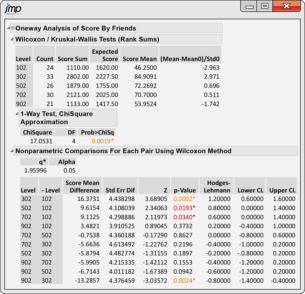
Figure 15.11 JMP output for the Kruskal-Wallis test applied to the Facebook data, Exercise 15.31.
 15.32 Jumping and strong bones. In Exercise 12.61 (page 646), you studied the effects of jumping on the bones of rats. Ten rats were assigned to each of three treatments: a 60-centimeter “high jump,” a 30-centimeter “low jump,” and a control group with no jumping.17 Here are the bone densities (in milligrams per cubic centimeter) after eight weeks of 10 jumps per day:
Group Bone density Control 611 621 614 593 593 653 600 554 603 569 Low jump 635 605 638 594 599 632 631 588 607 596 High jump 650 622 626 626 631 622 643 674 643 650 The study was a randomized comparative experiment. Outline the design of this experiment.
Make side-by-side stemplots for the three groups, with the stems lined up for easy comparison. The distributions are a bit irregular but not strongly non-Normal. We would usually use analysis of variance to assess the significance of the difference in group means.
Do the Kruskal-Wallis test. Explain the distinction between the hypotheses tested by Kruskal-Wallis and ANOVA.
Write a brief statement of your findings. Include a numerical comparison of the groups as well as your test result.
15.33 Do poets die young? In Exercise 12.60 (page 646) you analyzed the age at death for female writers. They were classified as novelists, poets, and nonfiction writers.

Use the Kruskal-Wallis test to compare the three groups of female writers.
Compare these results with what you find using the ANOVA F statistic.