15.1 The Wilcoxon Rank Sum Test
![]()
Two-sample problems (see Section 7.2) are among the most common in statistics. Here is an example of this setting.
Example 15.1 Does the American League get more hits?
![]()
In 1973, the American League adopted the designated-hitter rule, which allows a substitute player to take the place of the pitcher when it is the pitcher’s turn to bat. Because pitchers typically do not hit as well as other players, it was expected that the rule would produce more hits and, therefore, more excitement for the fans. The National League has not adopted this rule. Let’s look at some data to see if we can detect an increase in the number of hits per game between the American League and the National League. Here are the numbers of hits for eight games played on the same spring day, four from each league:
| League | Hits | |||
|---|---|---|---|---|
| American | 16 | 25 | 14 | 19 |
| National | 11 | 17 | 13 | 23 |
Let’s use this example to illustrate the basic ideas of nonparametric rank tests. The first step is to perform a transformation of the raw data, the eight observations in the data set. The transformation will replace the raw data by ranks. For a small data set, this can be done by hand. The rank transformation retains only the ordering of the observations and makes no other use of their numerical values. Working with ranks allows us to dispense with specific assumptions about the shape of the distribution, such as Normality.
The rank transformation
The first step in implementing this test is to rank all the data together. For a small data set, this can be done by hand. Here’s how.
Example 15.2 Ranks for the baseball data.
Let’s now rank the baseball hit data. Arrange the raw data in order from smallest to largest. Although we rank all the cases together, it is important to denote which observations are from each group. Here are the eight observations listed in order from smallest to largest:
The boldface entries in the list are the hits for the American League games. The idea of rank tests is to look just at position in this ordered list. We replace each observation by its order, from 1 (smallest) to 8 (largest). These numbers are the ranks:
| Hits | 11 | 13 | 14 | 16 | 17 | 19 | 23 | 25 |
| Rank | 1 | 2 | 3 | 4 | 5 | 6 | 7 | 8 |
It would not be unusual in the baseball example to have sampled from a day where more than one game had the same number of hits. We will discuss how to handle ties later in this section.
Check-in

15.1 Numbers of rooms in top meeting hotels. The software company Cvent ranks meeting hotels in the United States and lists the top 100, with characteristics of each hotel.1 We let Group A be the 25 top-ranked hotels and let Group B be the hotels ranked 26 to 50. A simple random sample of 5 hotels was taken from each group, and the number of rooms in each selected hotel was recorded. Here are the data:
Group A 1303 1522 2019 1260 1996 Group B 1564 1036 3933 1214 1096 Rank all the observations together and make a list of the ranks for Group A and Group B.

15.2 The effect of Caesars Palace on the result. Refer to the previous Check-in question. Caesars Palace in Las Vegas, with 3933 rooms, was the third hotel selected in Group B. Suppose, instead, a different hotel, with 1600 rooms, fewer than half as many, had been selected. Replace the observation 3933 in Group B with 1600. Use the modified data to make a list of the ranks for Groups A and B combined. What changes?

The Wilcoxon rank sum test
If the American League games have more hits than the National League games, we’d expect the ranks of the American League games to generally be higher than those of the National League games. Let’s compare the sums of these ranks for this example.
Example 15.3 Sum the ranks for the baseball data.
The following table gives the sum of the ranks presented in Example 15.2 for the games in each league:
| League | Sum of ranks |
|---|---|
| American | |
| National |
These sums compare the hits of the American League with those of the National League. In fact, the sum of the ranks from 1 to 8 is always equal to 36, so it is enough to report the sum for one of the two groups. Because the sum of the ranks for the American League is 21, the ranks for the National League must be 15 because
If there were no difference between the leagues, we would expect the sum of the ranks for each league to be 18 (half of the total sum of 36). The sum of the ranks is higher for the American League, but is this difference in ranks statistically significant? Here are the facts we need to complete the test for the general setting where the two samples need not be the same size.
Example 15.4 Hypotheses and test statistic for the baseball data.
For the baseball question in Example 15.1, we want to test
against the one-sided alternative
Our test statistic is the rank sum
Check-in
15.3 Hypotheses and test statistic for top hotels. Refer to Check-in question 15.1. State appropriate null and alternative hypotheses for this setting and calculate the value of W, the test statistic.
15.4 The effect of Caesars Palace on the test statistic. Refer to Check-in question 15.2. Using the altered data, state appropriate null and alternative hypotheses and calculate the value of W, the test statistic.
Example 15.5 Mean and standard deviation of W for the baseball data.
In Example 15.1,
and standard deviation
The observed sum of the ranks,
To calculate the P-value
The Normal approximation
The rank sum statistic W becomes approximately Normal as the two sample sizes increase. Thus, by standardizing W, we have a new z statistic:
Use standard Normal probability calculations to find P-values for this statistic. Because W takes only whole-number values, the continuity correction improves the accuracy of the approximation.
Example 15.6 Find and interpret the P-value.
The standardized rank sum statistic W in our baseball example is
We expect W to be larger when the alternative hypothesis is true, so the approximate P-value is
The continuity correction acts as if the whole number 21 occupies the entire interval from 20.5 to 21.5. We calculate the P-value
The data do not provide sufficient evidence to support our idea that American League games have more hits than National League games.
We have chosen
Example 15.7 Software output.
Figure 15.2 shows the Wilcoxon rank sum test output from JMP. The sum of the ranks for the American League is given as
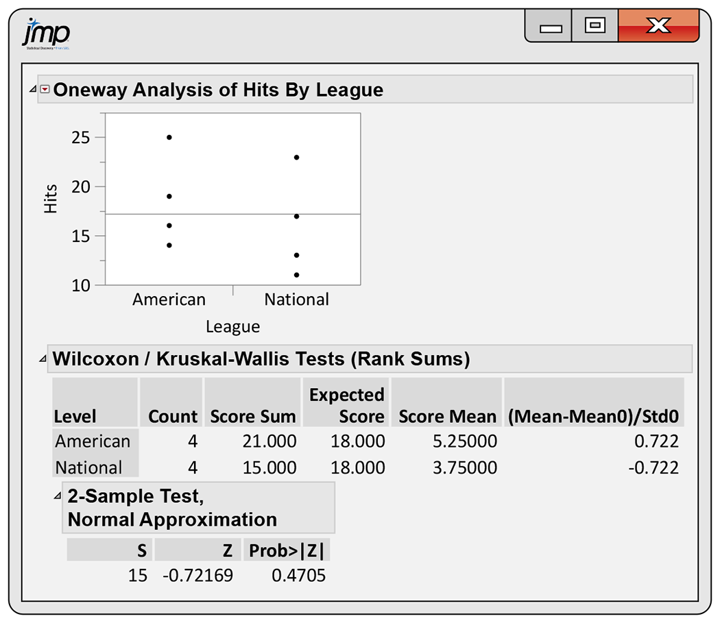
Figure 15.2 JMP output for the baseball hit data, Example 15.7.
Check-in
15.5 The P-value for top hotels. Refer to Check-in questions 15.1 and 15.3 (pages 15-4 and 15-6). Find
15.6 The effect of Caesars Palace on the P-value. Refer to Check-in questions 15.2 and 15.4 (pages 15-4 and 15-6). Perform the same analysis steps as in Check-in question 15.5 using the altered data. Do the altered data change the conclusion?
Example 15.8 More software output.
Figure 15.3 shows the test output for the baseball data from two additional statistical programs. Minitab gives the Normal approximation P-value, and it refers to the method as the Mann-Whitney test. This is an alternative form of the Wilcoxon rank sum test. It also reports the 95% confidence interval for the difference in medians. SPSS uses the exact calculation for the P-value. Both report the significance test for the two-sided alternative only.
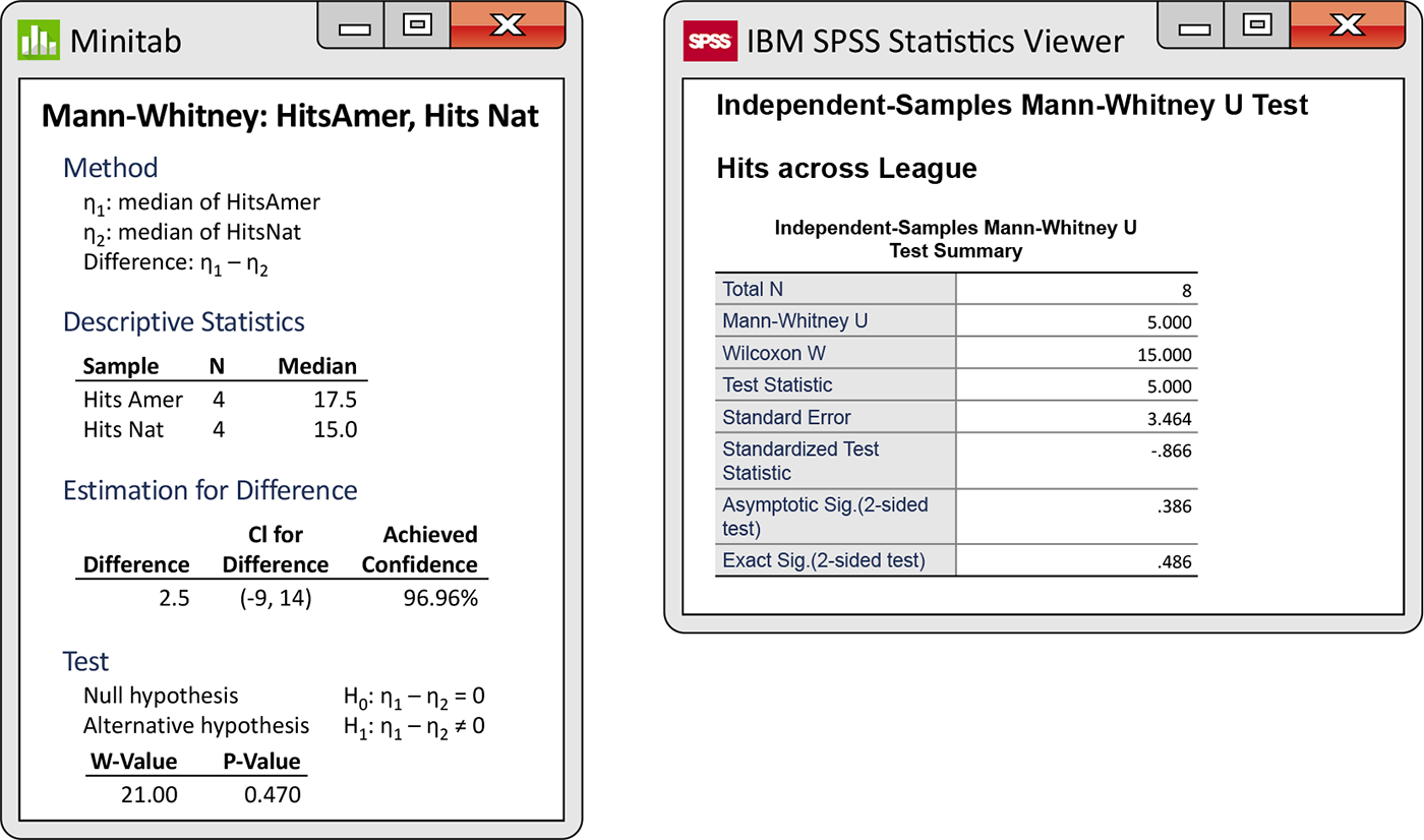
Figure 15.3 Minitab and SPSS outputs for the data in Example 15.8.
What hypotheses does Wilcoxon test?
Our null hypothesis is that the distribution of hits is the same in the two leagues. Our alternative hypothesis is that there are more hits in the American League than in the National League. If we are willing to assume that hits are Normally distributed, or if we have reasonably large samples, we use the two-sample t test for means. Our hypotheses then become
When the distributions may not be Normal, we might restate the hypotheses in terms of population medians rather than means:
![]() The Wilcoxon rank sum test does test hypotheses about population medians—but only if an additional assumption is met: the two populations must have distributions of the same shape and spread. That is, the density curve for hits in the American League must look exactly like that for the National League except that it may be shifted to the left or to the right.
The Wilcoxon rank sum test does test hypotheses about population medians—but only if an additional assumption is met: the two populations must have distributions of the same shape and spread. That is, the density curve for hits in the American League must look exactly like that for the National League except that it may be shifted to the left or to the right.
The same-shape assumption is too strict to be reasonable in practice. Recall that our preferred version of the two-sample t test does not require that the two populations have the same standard deviation—that is, it does not make a same-shape assumption. Fortunately, the Wilcoxon test also applies in a much more general and more useful setting. It tests hypotheses that we can state in words as
Here is a more exact statement of the systematically larger alternative hypothesis. Let
for any value of x.
Example 15.9 Systematically larger for baseball data.
Take
The alternative hypothesis says that this inequality holds not just for 15 hits but for any number of hits.
This exact statement of the hypotheses we are testing is a bit awkward.2 The hypotheses really are “nonparametric” because they do not involve any specific parameter, such as the mean or median. If the two distributions do have the same shape, the general hypotheses reduce to comparing medians. Many texts and computer outputs state the hypotheses in terms of medians, sometimes ignoring the same-shape requirement. We recommend that you express the hypotheses in words rather than symbols. “The number of American League hits per game is systematically higher than the number of National League hits per game” is easy to understand and is a proper statement of the effect that the Wilcoxon test examines.
Ties
The exact distribution for the Wilcoxon rank sum is obtained assuming that all observations in both samples take different values. This allows us to uniquely rank them. In practice, however, we often find observations tied at the same value. What shall we do? The usual practice is to assign all tied values the average of the ranks they occupy. Here is an example:
Example 15.10 Ties for the baseball data.
In Example 15.1 (page 15-3), we examined data where there were no ties but it would not be unlikely to see ties in samples like this. Let’s change the data so that the fourth entry for the National League is 25 instead of 23. Here is the resulting table:
| League | Hits | |||
|---|---|---|---|---|
| American | 16 | 25 | 14 | 19 |
| National | 11 | 17 | 13 | 25 |
Here are the ranked data, with the American League hits displayed in boldface.
To do this, replace each observation by its order. The following table summarizes the ranks for this altered data set. Notice that the two entries with 25 hits now share the rank 7.5. It is 7.5 because it is the average of 7 and 8, the two ranks these would have been given had they been unique. We strongly recommend using software to perform the test whenever there are ties.
| Hits | 11 | 13 | 14 | 16 | 17 | 19 | 25 | 25 |
| Rank | 1 | 2 | 3 | 4 | 5 | 6 | 7.5 | 7.5 |
The exact distribution for the Wilcoxon rank sum W changes if the data contain ties. Moreover, the standard deviation
It is sometimes useful to use rank tests on data that have very many ties because the scale of measurement has only a few values. Here is an example.
Example 15.11 Exergaming in Canada.
![]()

Exergames are active video games such as rhythmic dancing, virtual bicycles, balance board simulators, and virtual sports simulators that require a screen and a console. A study of exergaming in students from grades 10 and 11 in Montreal, Canada, examined many factors related to participation in exergaming.3 In Exercise 14.25 (page 14-21), we used logistic regression to examine the relationship between exergaming and time spent viewing television. Here are the data displayed in a two-way table of counts:
| Exergamer | TV time (hours per day) | ||
|---|---|---|---|
| None | Some but less than two hours | Two hours or more | |
| Yes | 6 | 160 | 115 |
| No | 48 | 616 | 255 |
How do we approach the analysis of these data using the Wilcoxon test? Before answering this, let’s perform a two-way table analysis.
Check-in
15.7 Analyze as a two-way table. Analyze the exergaming data in Example 15.11 as a two-way table.

Compute the percents in the three categories of TV watching for the exergamers. Do the same for those who are not exergamers. Display the percents graphically and summarize the differences in the two distributions.
- Perform the chi-square test for the counts in the two-way table. Report the test statistic, the degrees of freedom, and the P-value. Give a brief summary of what you can conclude from this significance test.
As with any other significance test, we start with the hypotheses. We have two distributions of TV viewing: one for the exergamers and one for those who are not exergamers. The null hypothesis states that these two distributions are the same. The alternative hypothesis uses the fact that the responses are ordered from no TV to two hours or more per day. It states that one of the groups watches more TV than the other.
The alternative hypothesis is two-sided. Because the responses can take only three values, there are very many ties. All
Example 15.12 Software output.
![]()
Look at Figure 15.4, which gives JMP output for the Wilcoxon test. The rank sum for the exergamers (using average ranks for ties) is
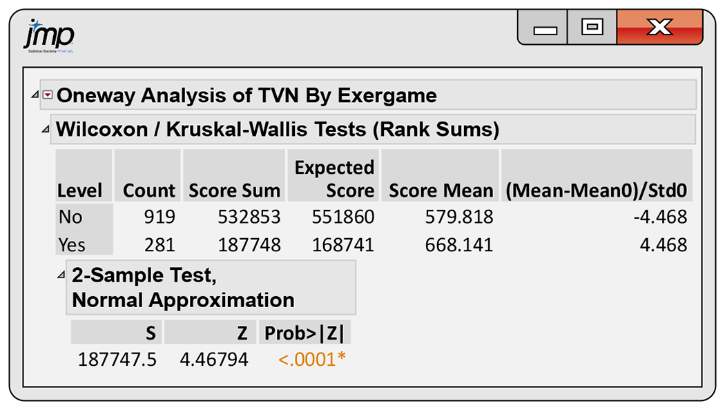
Figure 15.4 JMP output for the exergaming data, Example 15.12.
We can use our framework of “systematically larger” (page 15-9) to summarize these data. For the exergamers, 98% watch some TV and 41% watch two or more hours per day. The corresponding percents for the students who are not exergamers are 95% and 28%. The difference is statistically significant (
In our discussion of TV viewing and exergaming, we have expressed results in terms of the amount of TV watched. In fact, we do not have the actual hours of TV watched by each student in the study. Only data with the hours classified into three groups are available. Many government surveys summarize quantitative data categorized into ranges of values. ![]() When summarizing the analysis of data, it is very important to explain clearly how the data are recorded. In this setting, we have chosen to use phrases such as “watch more TV” because they express the findings based on the data available.
When summarizing the analysis of data, it is very important to explain clearly how the data are recorded. In this setting, we have chosen to use phrases such as “watch more TV” because they express the findings based on the data available.
Note that the two-sample t test would not be appropriate in this setting. If we coded the TV-watching categories as 1, 2, and 3, the average of these coded values would not be meaningful.
On the other hand, we frequently encounter variables measured in scales such as “strongly agree,” “agree,” “neither agree nor disagree,” “disagree,” and “strongly disagree.” In these circumstances, many would code the responses with the integers 1 to 5 and then use standard methods such as a t test or ANOVA. Whether to do this or not is a matter of judgment. Rank tests avoid the dilemma because they use only the order of the responses, not their actual values. ![]() Some statisticians use t procedures when there is not a fully meaningful scale of measurement, but others avoid them.
Some statisticians use t procedures when there is not a fully meaningful scale of measurement, but others avoid them.
Nonparametric rank and t procedures
The two-sample t procedures are the most commonly used procedures for comparing the centers of two populations based on random samples from each. The Wilcoxon rank sum test is a competing procedure that does not start from the condition that sample means have distributions that are approximately Normal. Tests based on Normality and nonparametric rank procedures apply in many other settings as well. How do these approaches compare in general?
- Moving from the actual data values to their ranks allows us to find an exact sampling distribution for rank statistics such as the Wilcoxon rank sum W when the null hypothesis is true. When our samples are small, are truly random samples from the populations, and show non-Normal distributions of the same shape, the Wilcoxon test is more reliable than the two-sample t test. In other situations, the robustness of t procedures implies that we can obtain reasonably accurate P-values.
- Normal tests compare means and are accompanied by simple confidence intervals for means or differences between means. When we use rank tests to compare medians, we can also give confidence intervals for medians. However, the usefulness of rank tests is clearest in settings when they do not simply compare medians; see the discussion “What hypotheses does Wilcoxon test?” (page 15-9). Rank methods focus on significance tests, not confidence intervals.
- Inference based on ranks is largely restricted to simple settings. Normal inference extends to methods for use with complex experimental designs and multiple regression, but nonparametric rank procedures do not. We stress Normal inference in part because it leads to more advanced statistics.
In general, Normal distribution methods are more useful than rank tests. ![]() We recommend rank tests only for very small samples that are clearly non-Normal. Other alternatives include the permutation and bootstrap methods discussed in Chapter 16.
We recommend rank tests only for very small samples that are clearly non-Normal. Other alternatives include the permutation and bootstrap methods discussed in Chapter 16.
Section 15.1 SUMMARY
- Nonparametric rank procedures do not require any specific form for the distribution of the population from which our samples come.
- Rank tests are nonparametric procedures based on the ranks of observations, their positions in the list, ordered from smallest (rank 1) to largest. Tied observations receive the average of their ranks.
- The Wilcoxon rank sum test compares two distributions to assess whether one has systematically larger values than the other. The Wilcoxon test is based on the Wilcoxon rank sum statistic W, which is the sum of the ranks of one of the samples. It is also called the Mann-Whitney test. The Wilcoxon test can replace the two-sample t test.
- P-values for the Wilcoxon rank sum test are based on the sampling distribution of the rank sum statistic W when the null hypothesis (no difference in distributions) is true. You can find P-values from special tables, software, or a Normal approximation (with continuity correction).
Section 15.1 EXERCISES
15.1 Time spent studying. A first-year college class had two large sections. One met at 8:30 a.m. (early), and the other met at 4:00 p.m. (late). A sample of 6 students from each section were interviewed about their class experience, including how much time they spent studying during a typical week day. Here are the responses, in minutes, for the students from the early section:

Here are the data for the students in the late section:
Combine the data for all 12 students and report the ranks.
15.2 Storytelling and the use of language. A study of early childhood education asked kindergarten students to retell two fairy tales that had been read to them earlier in the week. The 10 children in the study included five high-progress readers and five low-progress readers. Each child told two stories. Story 1 had been read to them; Story 2 had been read and also illustrated with pictures. An expert listened to a recording of each child and assigned a score for certain uses of language. Here are the data:4

Child Progress Story 1 score Story 2 score Child Progress Story 1 score Story 2 score 1 high 0.55 0.80 6 low 0.40 0.77 2 high 0.57 0.82 7 low 0.72 0.49 3 high 0.72 0.54 8 low 0.00 0.66 4 high 0.70 0.79 9 low 0.36 0.28 5 high 0.84 0.89 10 low 0.55 0.38 Is there evidence that the scores of high-progress readers are higher than those of low-progress readers when they retell a story they have heard without pictures (Story 1)?
Make Normal quantile plots for the five responses in each group. Are any major deviations from Normality apparent?
Carry out a two-sample t test. State hypotheses and give the two-sample means, the t statistic and its P-value, and your conclusion.
Carry out the Wilcoxon rank sum test. State hypotheses and give the rank sum W for high-progress readers, its P-value, and your conclusion. Do the t and Wilcoxon tests lead you to different conclusions?
15.3 Find the rank sum statistic for study times. Refer to Exercise 15.1. Compute the value of the Wilcoxon statistic. Take the first sample to be the students in the early section.
15.4 Repeat the analysis for Story 2. Repeat the analysis of Exercise 15.2 for the scores when children retell a story they have heard and seen illustrated with pictures (Story 2).
15.5 State the hypotheses for study times. Refer to Exercise 15.1. State appropriate null and alternative hypotheses for this setting.
15.6 Do the calculations by hand. Use the data in Exercise 15.2 for children telling Story 2 to carry out by hand the steps in the Wilcoxon rank sum test.
Arrange the 10 observations in order and assign ranks. There are no ties.
Find the rank sum W for the five high-progress readers. What are the mean and standard deviation of W under the null hypothesis that low-progress and high-progress readers do not differ?
Standardize W to obtain a z statistic. Do a Normal probability calculation with the continuity correction to obtain a one-sided P-value.
The data for Story 1 contain tied observations. What ranks would you assign to the 10 scores for Story 1?
15.7 Find the mean and standard deviation of the distribution of the statistic. The statistic W that you calculated in Exercise 15.3 is a random variable with a sampling distribution. What are the mean and the standard deviation of this sampling distribution under the null hypothesis?
15.8 Is civic engagement related to education? A Pew Internet Poll of adults aged 18 and older examined factors related to civic engagement. Participants were asked whether or not they had participated in a civic group or activity in the preceding 12 months. One analysis looked at the relationship between this variable and education. Here are the data:5

Civic participation Education No high school High school Some college College Civic 76 294 295 428 No civic 155 424 273 298 Figure 15.5 gives the JMP output for analyzing these data using the Wilcoxon rank sum test.
Describe the relevant parts of the output and write a short summary of the results.
Apply the “systematically larger” framework that we used in Example 15.9 (page 15-9) to these data. Is this a useful way to describe the results of this analysis? Give reasons for your answer.
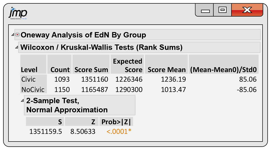
Figure 15.5 JMP output for the civic participation data, Exercise 15.8.
15.9 Find and interpret the P-value. Refer to the odd-numbered exercises from Exercises 15.1 through Exercise 15.7. Find the P-value using the Normal approximation with the continuity correction and interpret the result of the significance test.
15.10 Do women talk more? Conventional wisdom suggests that women are more talkative than men. One study designed to examine this stereotype collected data on the speech of 10 men and 10 women in the United States.6 The variable recorded is the number of words per day. Here are the data:

Men Women 23,871 5,180 9,951 12,460 10,592 24,608 13,739 22,376 17,155 10,344 9,811 12,387 9,351 7,694 16,812 21,066 29,920 21,791 32,291 12,320 Summarize the data for the two groups, using numerical and graphical methods. Describe the two distributions.
Compare the words per day spoken by the men with the words per day spoken by the women using the Wilcoxon rank sum test. Summarize your results and conclusion in a short paragraph.
15.11 More data for women and men talking. The data in the previous exercise were a sample of the data collected in a larger study of 42 men and 37 women. Use the larger data set to answer the questions in the previous exercise. Discuss the advisability of using the Wilcoxon rank sum test versus the t test for this exercise and for the previous one.

 15.12 Learning math through subliminal messages. A “subliminal” message is below our threshold of awareness but may, nonetheless, influence us. Can subliminal messages help students learn math? A group of students who had failed the mathematics part of the City University of New York Skills Assessment Test agreed to participate in a study to find out. All received a daily subliminal message, flashed on a screen too rapidly to be consciously read. The treatment group of 10 students was exposed to the message “Each day I am getting better in math.” The control group of eight students was exposed to the neutral message “People are walking on the street.” All students participated in a summer program designed to raise their math skills, and all took the assessment test again at the end of the program. Here are data on the subjects’ scores before and after the program:7
Treatment group Control group Pretest Posttest Pretest Posttest 18 24 18 29 18 25 24 29 21 33 20 24 18 29 18 26 18 33 24 38 20 36 22 27 23 34 15 22 23 36 19 31 21 34 17 27 The study design was a randomized comparative experiment. Outline this design.
Compare the gain in scores in the two groups, using a graph and numerical descriptions. Does it appear that the treatment group’s scores rose more than the scores for the control group?
Apply the Wilcoxon rank sum test to the posttest versus pretest differences. Note that there are some ties. What do you conclude?