2.2 Scatterplots
![]()
Example 2.9 Laundry detergents.
![]()
Consumers Union provides ratings on a large variety of consumer products. It uses sophisticated testing methods as well as surveys of its members to create these ratings, which it publishes in its magazine, Consumer Reports.4
One recent study rated 53 laundry detergents on a scale from 1 to 100. The scale summarizes washing performance under a variety of conditions. Price per load is given in cents.5 We will examine the relationship between rating and price per load for these laundry detergents.
What should this relationship look like? Should we expect higher-priced detergents to have higher ratings? Or might the rating drop if the cost per load gets too high? Our first step is to look at the data set.
Check-in
-
2.5 Examine the spreadsheet. Examine the spreadsheet of the laundry detergent data.

-
How many cases are in the data set?
-
Describe the labels, variables, and values.
-
Which columns represent quantitative variables? Which columns represent categorical variables?
-
Is there an explanatory variable? A response variable? Explain your answer.
-
-
2.6 Use the data set. Using the data set from the previous Check-in question, create graphical and numerical summaries for the variables Rating and Price.
Now that we have an understanding of the data set, let’s study the relationship. We begin with a graphical display. The most common way to display the relationship between two quantitative variables is by using a scatterplot. It helps us to describe the form and strength of the association.
Example 2.10 Scatterplot for laundry detergents.
![]()
A higher price for a product should be associated with a better product. Therefore, in our examination of the relationship, let’s treat price per load, expressed in cents, as the explanatory variable and rating as the response variable in our examination of the relationship between these two variables. We begin with a graphical display.
Figure 2.1 gives a scatterplot that displays the relationship between the response variable, rating, and the explanatory variable, price per load. The most striking feature that we see in the plot is a case that appears to be very different from the others. One of the laundry detergents has a rating that is about average (51), but the price per load (56 cents) is almost double that of the other products.
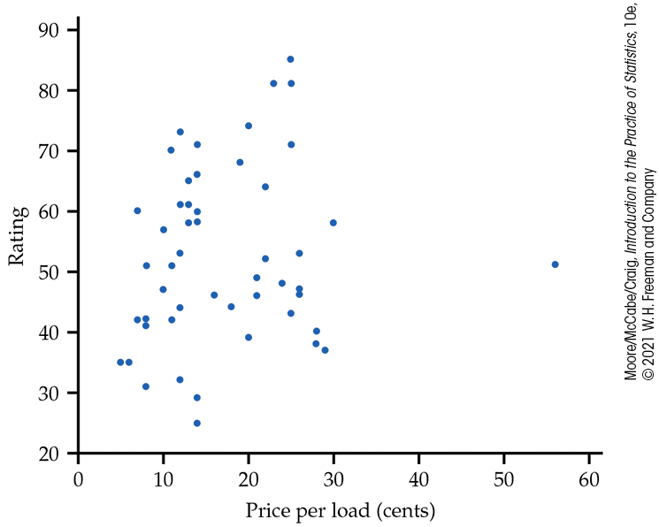
Figure 2.1 Scatterplot of rating versus price per load (in cents) for 53 laundry detergents, Example 2.10.
Cases that fall well outside the general pattern of the relationship are called outliers. We provide a more detailed description of these in Section 2.5. For now, we remove this case and focus on the relationship of the remaining data.
Figure 2.2 gives the scatterplot with the outlier removed. It might be the case that a higher price is associated with a higher rating but the association is weak. Paying a high price for your laundry detergent will not guarantee that you have selected a highly rated product.
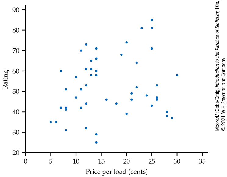
Figure 2.2 Scatterplot of rating versus price per load (in cents) for 52 laundry detergents (with the outlier removed), Example 2.10.
Always plot the explanatory variable, if there is one, on the horizontal axis (the x axis) of a scatterplot. We usually call the explanatory variable x and the response variable y. If there is no explanatory–response distinction, either variable can go on the horizontal axis. Time plots such as the one in Figure 1.11 (page 20) are special scatterplots where the explanatory variable x is a measure of time.
Check-in
-
2.7 Make a scatterplot. Let’s consider the laundry data with the outlier removed.

-
Make a scatterplot similar to Figure 2.2.
-
Two of the laundry detergents cost 14 cents per load and have a rating of 60. Mark the location of these items on your plot.
-
Cases with identical values for both variables are generally indistinguishable in a scatterplot. To what extent do you think that this could give a distorted picture of the relationship between two variables for a data set that has a large number of duplicate values? Explain your answer.
-
An option called jitter is available with some statistical software that will add a little noise to each point so that points with identical values will appear to be different. If you have software that includes this option, apply it to your plot and summarize the effect of the jittering.
-
-
2.8 Change the units. Refer to the laundry data with the outlier.
-
Create a spreadsheet for the laundry detergent data with the price per load expressed in dollars.
-
Make a scatterplot for the data in your spreadsheet.
-
Describe how this scatterplot differs from Figure 2.2.
-
Interpreting scatterplots
To look more closely at a scatterplot such as Figure 2.2, apply the strategies of exploratory analysis learned in Chapter 1. Instead of shape, center, and spread for distributions, we will look at form, direction, and strength for relationships.
The relationship in Figure 2.2 is difficult to see. But when we look at it carefully, we see that it suggests a linear relationship. In other words, it may be appropriate to summarize the relationship with a straight line. To explore this possibility, we can use software to put a straight line through the data. We will see more details about how this is done in Section 2.4 (page 98).
Example 2.11 Scatterplot with a straight line.
![]()
Figure 2.3 plots the laundry detergent data with a straight line. The line helps us to see and to evaluate the linear form of the relationship.
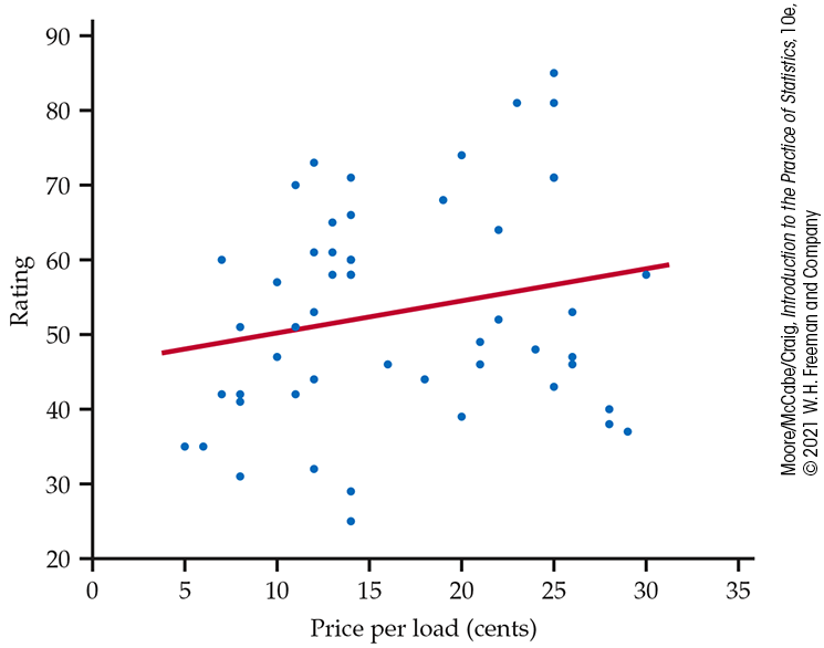
Figure 2.3 Scatterplot of rating versus price per load (in cents) with a fitted straight line, Example 2.11.
There is a large amount of scatter about the line. Referring to the data file LAUND, we see that there are eight laundry detergents with a price of 14 cents per load. For these products, the variation in ratings is substantial, from 25 to 71. We do not see any additional outliers in this plot.
Although it is very weak, the relationship in Figure 2.3 has a direction: laundry detergents that cost more have somewhat higher ratings. This is a positive association between the two variables.
The strength of a relationship in a scatterplot is determined by how closely the points follow a clear form. The overall relationship in Figure 2.3 is weak. Here is an example of a stronger linear relationship.
Example 2.12 Education spending and population: Benchmarking.
![]()
We expect that states with larger populations would spend more on education than states with smaller populations.6 What is the nature of this relationship? Can we use this relationship to evaluate whether some states are spending more than we expect or less than we expect? The basic idea is to compare processes or procedures of an organization with those of similar organizations. This type of exercise is called benchmarking.
Figure 2.4 is a spreadsheet giving the education spending and the populations of the 50 U.S. states. Figure 2.5 is a scatterplot of the education spending versus the population with a straight line. The scatterplot shows a strong positive relationship between these two variables.
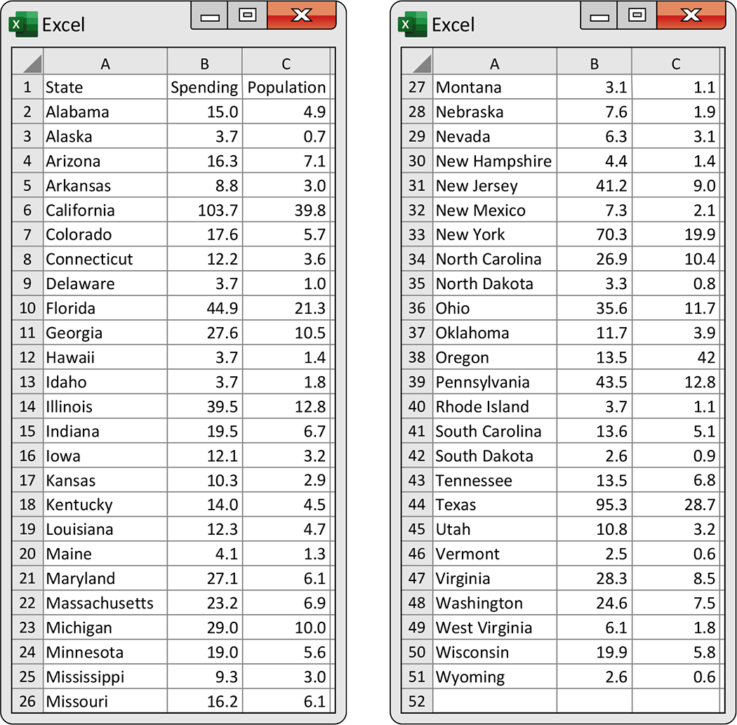
Figure 2.4 Spending (in billions of dollars) and population (in millions) for the 50 U.S. states, Example 2.12.
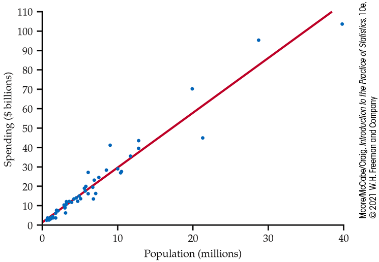
Figure 2.5 Scatterplot of spending ($ billion) versus population (in millions) for the 50 U.S. states, with a fitted straight line, Example 2.12.
Check-in
-
2.9 Make a scatterplot. In our Mocha Frappuccino® example (Example 2.2, page 73), the 12-ounce drink costs $4.75, the 16-ounce drink costs $5.25, and the 24-ounce drink costs $5.75. Explain which variable should be used as the explanatory variable and make a scatterplot and include the fitted straight line if your software includes this option. Describe the scatterplot and the association between these two variables.
Of course, not all relationships are linear. Here is an example where a relationship is described by a curve.
Example 2.13 Calcium retention.
![]()
Our bodies need calcium to build strong bones. How much calcium do we need? Does the amount that we need depend on our age? Nutrition researchers study questions like these. One series of studies used the amount of calcium retained by the body as a response variable and the amount of calcium consumed as an explanatory variable.7
Figure 2.6 is a scatterplot of calcium retention in milligrams per day (mg/d) versus calcium intake (mg/d) for 56 children aged 11 to 15 years. A smooth curve generated by software helps us see the relationship between the two variables.
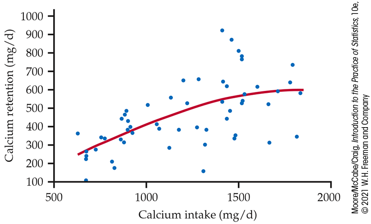
Figure 2.6 Scatterplot of calcium retention (mg/d) versus calcium intake (mg/d) for 56 children with a smooth curve, Example 2.13. The relationship is positive, but it is not linear.
There is clearly a relationship here. As calcium intake increases, the body retains more calcium. However, the relationship is not linear. The curve is approximately linear for low values of intake, but then the line curves more and becomes almost level.
There are many kinds of curved relationships like that in Figure 2.6. For some of these, we can apply a transformation to the data that will make the relationship approximately linear. To do this, we replace the original values with the transformed values and then use the transformed values for our analysis.
Transforming data is common in statistical practice. There are systematic principles that describe how transformations behave and guide the search for transformations that will, for example, make a distribution more Normal or a curved relationship more linear.
The log transformation
The most important transformation that we will use is the log transformation. This transformation can be used for variables that have positive values only. Occasionally, we use it when there are zeros, but in this case, we first replace the zero values with some small value, often one-half of the smallest positive value in the data set.
You have probably encountered logarithms in one of your high school mathematics courses as a way to do certain kinds of arithmetic. Logarithms are a powerful tool when used in statistical analyses. We will use natural logarithms. Statistical software and statistical calculators generally provide easy ways to perform this transformation.
Let’s try a log transformation on our calcium retention data. Here are the details.
Example 2.14 Calcium retention with logarithms.
![]()
Figure 2.7 is a scatterplot of the log of calcium retention versus calcium intake. The plot includes a fitted straight line to help us see the relationship. We see that the transformation has worked. Our relationship is now approximately linear.
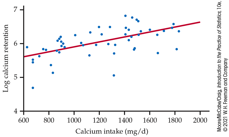
Figure 2.7 Scatterplot of the log of calcium retention versus calcium intake for 56 children, with a fitted line, Example 2.14. The relationship is approximately linear.
Our analysis of the calcium retention data in
Examples 2.13 and
2.14 reminds us of an
important issue when describing relationships. In
Example 2.13, we noted
that the relationship appeared to become approximately flat.
Biological processes are consistent with this observation. There is
probably a point where additional intake does not result in any
additional retention. With our transformed relationship in
Figure 2.7, however, there
is no leveling off as we saw in
Figure 2.6, even though we
appear to have a good fit to the data. The relationship and fit apply
to the range of data that are analyzed.
![]() We cannot assume that the relationship between two variables
extends beyond the range of the data.
We cannot assume that the relationship between two variables
extends beyond the range of the data.
For the calcium data, we used a log transformation of the response variable to describe the curved relationship in Figure 2.6 as the linear relationship in Figure 2.7. Here is another application but with the log transformation applied to both variables.
Example 2.15 Education spending and population with logarithms.
![]()
Let’s examine the relationship between spending and population, using logs for both variables. Figure 2.8 gives the plot with the fitted line.
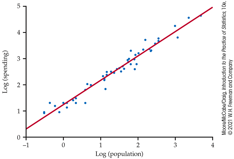
Figure 2.8 Scatterplot of log spending versus log population for the 50 U.S. states, with a fitted line, Example 2.15. The relationship is approximately linear.
Check-in
-
2.10 Compare the plots. Compare the plot in Figure 2.8 with the one in Figure 2.5 (page 82). Which one do you prefer? Give reasons for your answer.

Use of transformations and the interpretation of scatterplots are arts
that require judgment and knowledge about the variables that we are
studying.
![]() Always ask yourself if the relationship that you see makes
sense.
If it does not, then additional analyses are needed to understand the
data.
Always ask yourself if the relationship that you see makes
sense.
If it does not, then additional analyses are needed to understand the
data.
Adding categorical variables to scatterplots
![]()
In Figure 2.3 (page 80), we looked at the relationship between the rating and the price per load for 52 laundry detergents (outlier excluded). A more detailed look at the data shows that there are two different types of laundry detergent included in this data set: liquid and powder. Let’s examine where these two types of laundry detergents are in our plot.
Example 2.16 Rating versus price and type of laundry detergent.
![]()
In Figure 2.9, our scatterplot uses blue for liquids and red for powders. Separate lines are given for each type of laundry detergent. Most of the laundry detergents are liquids. There are three powders with somewhat low prices and four powders with relatively high prices. The prices of the powders are similar to the prices of the liquids.
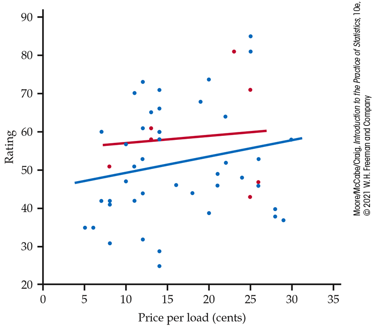
Figure 2.9 Scatterplot of rating versus price per load (in cents), with fitted straight lines, for 52 laundry detergents, Example 2.16. The type of detergent is indicated by the color: blue for liquid and red for powder.
In this example, we used a categorical variable, Type, to distinguish the two types of laundry detergents in our plot. Suppose that the additional variable that we want to investigate is quantitative. In this situation, we sometimes can combine the values into ranges of the quantitative variable—such as high, medium, and low—to create a categorical variable.
![]() Careful judgment is needed in using scatterplots. Don’t be
discouraged if your first attempt is not very successful. In
performing a good data analysis, you will often produce several plots
before you find the one that you believe to be the most effective in
describing the data.8
Careful judgment is needed in using scatterplots. Don’t be
discouraged if your first attempt is not very successful. In
performing a good data analysis, you will often produce several plots
before you find the one that you believe to be the most effective in
describing the data.8
Scatterplot smoothers
In Figure 2.6 (page 82), we added a smooth curve to our scatterplot to better understand the relationship between calcium retention and calcium intake. This curve helped us to see that the amount of calcium retained tends to level off as the intake increases. The method that we used to construct the curve is called smoothing.
Today, most statistical software includes options to perform the calculations needed for smoothing. The technical details vary, but the basic idea is that there is a smoothing parameter that controls the degree to which the relationship is smoothed. Here is another example.
Example 2.17 Laundry rating versus price with a smooth fit.
![]()
Figure 2.2 (page 79) gives the scatterplot for rating versus price for the remaining 52 laundry detergents that we studied in Example 2.9. In Figure 2.3, we added a straight line to the plot to help us see the relationship. Figure 2.10 shows the laundry detergent with two different smooth curves. The first (a) used a relatively small value of the smoothing parameter. The second (b) used a larger value, making the curve smoother. Overall, the relationship is very weak, and there is no clear pattern in the plot.
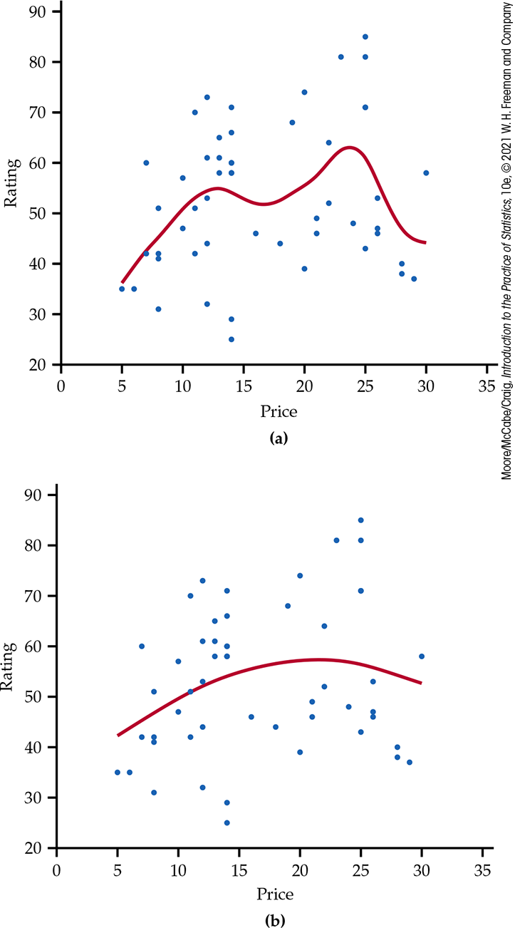
Figure 2.10 Scatterplot of rating versus price per load (in cents), with smooth curves, Example 2.17: (a) with a small value of the smoothing parameter; (b) with a higher value of the smoothing parameter.
Scatterplot smoothers can help you learn about relationships between two quantitative variables. They can confirm that there is a linear relationship, or they can suggest other features that are not evident from a casual look at the scatterplot. Here is an example of the latter scenario.
Example 2.18 A smooth fit for education spending and population with logs.
![]()
Figure 2.11 gives the scatterplot of log education spending versus log population for a previous year with a smooth curve. The curve suggests that the relationship is approximately linear except for states with relatively small populations. For these, the spending is relatively flat.
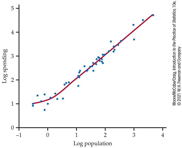
Figure 2.11 Scatterplot of log spending versus log population, with a smooth curve fitted to the data, for the 50 U.S. states, Example 2.18. This smooth curve fits the data very well and suggests that the relationship is generally linear except for states with small populations.
Categorical explanatory variables
A scatterplot displays the association between two quantitative variables. To display a relationship between a categorical variable and a quantitative variable, make a side-by-side comparison of the distributions of the response for each category. Back-to-back stemplots (page 13) and side-by-side boxplots (page 34) are useful tools for this purpose.
We will study methods for describing the association between two categorical variables in Section 2.6 (page 128).
Section 2.2 SUMMARY
-
A scatterplot displays the relationship between two quantitative variables. Mark values of one variable on the horizontal axis (x axis) and values of the other variable on the vertical axis (y axis). Plot each case’s data as a point on the graph.
-
Always plot the explanatory variable, if there is one, on the x axis of a scatterplot. Plot the response variable on the y axis.
-
In examining a scatterplot, look for an overall pattern showing the form, direction, and strength of the relationship and then look for outliers or other deviations from this pattern.
-
Form: Linear relationships, where the points show a straight-line pattern, are an important form of relationship between two variables. Curved relationships are also quite common.
-
Direction: If the relationship has a clear direction, we speak of either positive association (high values of the two variables tend to occur together) or negative association (high values of one variable tend to occur with low values of the other variable).
-
Strength: The strength of a relationship is determined by how close the points in the scatterplot lie to a simple form such as a line.
-
Plot points with different colors or symbols to see the effect of a categorical variable in a scatterplot.
-
To display the relationship between a categorical explanatory variable and a quantitative response variable, make a graph that compares the distributions of the response variable for each category of the explanatory variable.
-
A log transformation of one or both variables in a scatterplot can help us to understand the relationship between two quantitative variables.
-
A scatterplot smoother is a tool to examine the relationship between two quantitative variables by fitting a smooth curve to the data. The amount of smoothing can be varied using a smoothing parameter.
Section 2.2 EXERCISES
-
2.6 Make some sketches. For each of the following situations, make a scatterplot that illustrates the given relationship between two variables.
-
A weak negative linear relationship.
-
No apparent relationship.
-
A strong positive relationship that is not linear.
-
A more complicated relationship. Explain the relationship.
-
-
2.7 What’s wrong? Explain what is wrong with each of the following:
-
In a scatterplot, we put the response variable on the x axis and the categorical variable on the y axis.
-
If two variables are positively associated, then high values of one variable are associated with low values of the other variable.
-
A histogram can be used to examine the relationship between two variables.
-
-
2.8 Blueberries and anthocyanins. Anthocyanins are compounds that appear to have some health benefits for bones, the heart, and the brain. Blueberries are a good source of many different anthocyanins. Researchers at the Piedmont Research Station of North Carolina State University have assembled a database giving the concentrations of 18 different anthocyanins for 267 varieties of blueberries.9 Four of the anthocyanins measured are delphinidin-3-arabinoside, malvidin-3-arabinoside, cyanidin-3-galactoside, and delphinidin-3-glucoside, all measured in units of mg per 100 g of berries (dry weight). In the data file, we have simplified the names of these anthocyanins to Antho1, Antho2, Antho3, and Antho4.

-
Make a scatterplot of the data with Antho4 on the x axis and Antho3 on the y axis.
-
Describe the form, direction, and strength of the relationship.
-
Are there any outliers or unusual observations?
-
Is it useful to add a straight line to your scatterplot? Explain your answer.
-
If you have access to the appropriate software, explore the use of a scatterplot smoother to understand this relationship. Summarize what you have found using this method.
-
-
2.9 Blueberries and anthocyanins with logs. Refer to the previous exercise. In Exercises 1.124 and 1.125 (page 69), you examined the distributions of Antho3 and Antho4. Transform each of the variables with a log, make a scatterplot, and answer the questions in the previous exercise for the transformed data.
-
2.10 Blueberries and anthocyanins: Raw data or logs. Refer to Exercises 2.8 and 2.9.
-
Compare your results from the two exercises.
-
For exploring and explaining the relationship between Antho4 and Antho3, do you prefer the analysis you performed in Exercise 2.8 or the one you performed in Exercise 2.9? Give reasons for your answer.
-
-
2.11 Fuel consumption. Natural Resources Canada tests new vehicles each year and reports several variables related to fuel consumption for vehicles in different classes.10 For 2018 the group provides data for 502 vehicles that use regular fuel. Two variables reported are carbon dioxide

-
Make a scatterplot of the data with highway fuel consumption on the x axis and
-
Describe the form, direction, and strength of the relationship.
-
Are there any outliers or unusual observations?
-
-
2.12 Fuel consumption with a line. Refer to the previous exercise.
-
Add a line to the plot. To what extent to you think that the line does a good job of summarizing the relationship?
-
If your have the appropriate software, use smooth curves to examine the relationship. Does your analysis support the idea of using a straight line to summarize the relationship? Summarize what you find using this method.
-
-
2.13 Fuel consumption for different types of vehicles. Refer to the previous two exercises. Those exercises examined data for vehicles that used regular fuel. Data are also available for vehicles that use several other types of fuel. There are 1045 vehicles in total. The variable Fuel has four different possible values: X, for regular fuel; Z, for premium fuel; D, for diesel; and E, for ethanol.

-
Make a scatterplot of all of the data using different symbols or colors for the different fuel types.
-
Does the relationship between
-
-
2.14 Bone strength. Osteoporosis is a condition where bones become weak. It affects more than 200 million people worldwide. Exercise is one way to produce strong bones and to prevent osteoporosis. Because we use our dominant arm (the right arm for most people) more than our nondominant arm, we expect the bone in our dominant arm to be stronger than the bone in our nondominant arm. By comparing the strengths, we can get an idea of the effect that exercise can have on bone strength. Here are some data on the strength of bones, measured in Newton meters divided by 1000 (Nm/1000), for the arms of 15 young men (Group=“Control”):11

ID Nondominant Dominant ID Nondominant Dominant 1 15.7 16.3 9 15.9 20.1 2 25.2 26.9 10 13.7 18.7 3 17.9 18.7 11 17.7 18.7 4 19.1 22.0 12 15.5 15.2 5 12.0 14.8 13 14.4 16.2 6 20.0 19.8 14 14.1 15.0 7 12.3 13.1 15 12.3 12.9 8 14.4 17.5 Before attempting to compare the arm strengths of the nondominant and dominant arms, let’s take a careful look at the data for these two variables.
-
Make a scatterplot of the data with the nondominant arm strength on the x axis and the dominant arm strength on the y axis.
-
Describe the overall pattern in the scatterplot and any striking deviations from the pattern.
-
Describe the form, direction, and strength of the relationship.
-
Identify any outliers.
-
Is the relationship approximately linear?
-
-
2.15 Bone strength for baseball players. Refer to the previous exercise. The study collected arm bone strength information for two groups of young men. The data in the previous exercise were for a control group. The second group (Group=“Baseball”) in the study comprised men who played baseball. We know that these baseball players use their dominant arm in throwing (those who throw with their nondominant arm were excluded), so they get more arm exercise than the controls. Here are the data for the baseball players:
ID Nondominant Dominant ID Nondominant Dominant 16 17.0 19.3 24 15.1 19.4 17 16.9 19.0 25 13.5 20.4 18 17.7 25.2 26 13.6 17.1 19 21.2 37.7 27 20.3 26.5 20 21.0 40.3 28 17.3 30.3 21 14.6 20.8 29 14.6 17.4 22 31.5 36.9 30 22.6 35.0 23 14.9 21.2 Answer the questions in the previous exercise for the baseball players.
-
2.16 Compare the baseball players with the controls. Refer to the previous two exercises.
-
Plot the data for the two groups on the same graph, using different symbols for the baseball players and the controls.
-
Use your plot to describe and compare the relationships for the two variables. Write a short paragraph summarizing what you have found.
-
-
2.17 Graduation in four years and undergraduate major. How well does your undergraduate major predict the chance that you will graduate in four years? Data for a sample of 1200 recent college graduates were analyzed to address this question. What are the explanatory and response variables? Are these variables categorical or quantitative? Can the methods discussed in this section be used to analyze these data? Explain your answer.
-
2.18 What’s in the beer? The website beer100.com advertises itself as “Your Place for All Things Beer.” One of their “things” is a list of 160 domestic beer brands with the percent alcohol, calories per 12 ounces, and carbohydrates per 12 ounces (in grams).12

-
Figure 2.12 gives a scatterplot of calories versus percent alcohol. Give a short summary of what can be learned from the plot.
-
One of the points is an outlier. Find the brand of the outlier. How is this brand of beer different from the other brands?
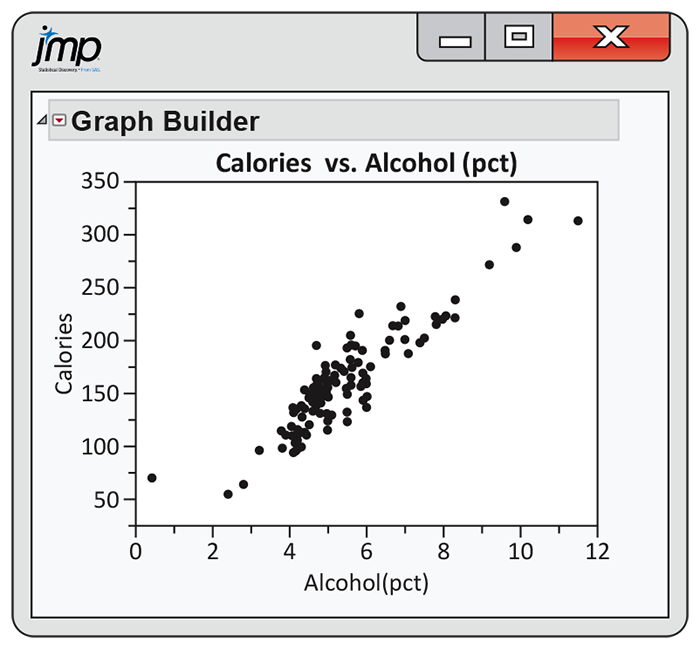
Figure 2.12 Scatterplot of calories versus percent alcohol for 160 domestic brands of beer, Exercise 2.18.

-
-
2.19 More beer. Refer to the previous exercise.
-
Make a scatterplot of calories versus percent alcohol using the data set without the outlier.
-
Describe the relationship between these two variables. If your software is capable, use a line and smoothers to explore the relationship.
-
-
2.20 Imported beer. The beer100.com website also gives data for imported beers. Describe the relationship between calories and percent alcohol for these imported beers. Use percent alcohol as the explanatory variable and calories as the response variable.

-
2.21 Compare domestic with imported. Plot calories versus percent alcohol for domestic and imported beers on the same scatterplot. Use different colors or symbols for the two types of beers. Summarize what this plot tells you about the relationship and the difference between the two types of beer. In particular, note any characteristics that are better shown in this plot relative to what was learned in Exercises 2.18, 2.19, and 2.20.

-
2.22 Decay of a radioactive element. Barium-137m is a radioactive form of the element barium that decays very rapidly. It is easy and safe to use for lab experiments in schools and colleges.13 In a typical experiment, the radioactivity of a sample of barium-137m is measured for one minute. It is then measured for three additional one-minute periods, separated by two minutes. So data are recorded at one, three, five, and seven minutes after the start of the first counting period. The measurement units are counts. Here are the data for one of these experiments:14

Time 1 3 5 7 Count 578 317 203 118 -
Make a scatterplot of the data. Give reasons for the choice of which variables to use on the x and y axes.
-
Describe the overall pattern in the scatterplot and any striking deviations from the pattern.
-
Describe the form, direction, and strength of the relationship.
-
Identify any outliers.
-
Is the relationship approximately linear?
-
-
2.23 Use a log for the radioactive decay. Refer to the previous exercise. Transform the counts using a log transformation. Then repeat parts (a) through (e) for the transformed data and compare your results with those from the previous exercise.
-
2.24 Internet use and babies. The World Bank collects data on many variables related to world development for countries throughout the world. Two of these variables are Internet use, in number of users per 100 people, and births per 1000 people.15 Figure 2.13 is a scatterplot of birth rate versus Internet use for the 106 countries that have data available for both variables.

-
Describe the relationship between these two variables.
-
A friend looks at this plot and concludes that using the Internet will decrease the number of babies born. Write a short paragraph explaining why the association seen in the scatterplot does not provide a reason to draw this conclusion.
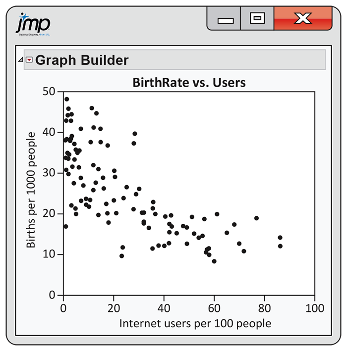
Figure 2.13 Scatterplot of births (per 1000 people) versus Internet users (per 100 people) for 106 countries, Exercise 2.24.
-
-
2.25 Try a log. Refer to the previous exercise.
-
Make a scatterplot of the log of births per 1000 people versus Internet users per 100 people.
-
Describe the relationship that you see in this plot and compare it with Figure 2.13.
-
Which plot do you prefer? Give reasons for your answer.
-
-
2.26 Make another plot. Refer to Exercise 2.24.
-
Make a new data set that has Internet users expressed as users per 10,000 people and births as births per 10,000 people.
-
Explain why these transformations to give new variables are linear transformations. (Hint: See linear transformations on page 40.)
-
Make a scatterplot using the transformed variables.
-
Compare your new plot with the one in Figure 2.13.
-
Why do you think that the analysts at the World Bank chose to express births as births per 1000 people and Internet users as users per 100 people?
-
-
2.27 Body mass and metabolic rate. Metabolic rate, the rate at which the body consumes energy, is important in studies of weight gain, dieting, and exercise. The following table gives data on the lean body mass and resting metabolic rate for 12 women and 7 men who are subjects in a study of dieting. Lean body mass, given in kilograms, is a person’s weight without fat. Metabolic rate is measured in calories burned per 24 hours, the same calories used to describe the energy content of foods. The researchers believe that lean body mass is an important influence on metabolic rate.

Subject Sex Mass Rate Subject Sex Mass Rate 1 M 62.0 1792 11 F 40.3 1189 2 M 62.9 1666 12 F 33.1 913 3 F 36.1 995 13 M 51.9 1460 4 F 54.6 1425 14 F 42.4 1124 5 F 48.5 1396 15 F 34.5 1052 6 F 42.0 1418 16 F 51.1 1347 7 M 47.4 1362 17 F 41.2 1204 8 F 50.6 1502 18 M 51.9 1867 9 F 42.0 1256 19 M 46.9 1439 10 M 48.7 1614 -
Make an appropriate scatterplot with lean body mass as the explanatory variable and resting metabolic rate as the response variable. Use different symbols or colors for men and women.
-
Is the association between these variables positive or negative? What is the form of the relationship? How strong is the relationship?
-
Does the pattern of the relationship differ for women and men? How do the male subjects as a group differ from the female subjects as a group?
-