6.2 Tests of Significance
The confidence interval is appropriate when our goal is to estimate population parameters. The second common type of inference is directed at a different goal: to assess the evidence provided by the data in favor of some claim about the population parameters. Assessing the randomness of tree locations in a forest in Example 6.1 (page 329) and the effectiveness of a new oral antibiotic in Example 6.2 (page 330) are two examples of this type of inference.
The reasoning of significance tests
A significance test is a formal procedure for comparing observed data with a hypothesis whose truth we want to assess. The hypothesis is a statement about the population parameters. The results of a test are expressed in terms of a probability that measures how well the data and the hypothesis agree. We use the following examples to illustrate these concepts.
Example 6.8 Grants and scholarships amount by planner status.
One purpose of Sallie Mae’s annual study described in Example 6.4 (page 336) is to allow comparisons of different subgroups. For example, in the latest report, 882 of the 2000 respondents (44.1%) had a plan in place to pay for all years of school before the student enrolled. The average grants and scholarships amount among them was $8460. The average grants and scholarships amount among those who did not have a plan was $7949. The difference of $511 is fairly large, but we know that these numbers are estimates of the population means. If we took different samples, we would get different estimates.
Can we conclude from these data that the average grants and scholarships amounts in these two groups are different? One way to answer this question is to compute the probability of obtaining a difference as large as or larger than the observed $511, assuming that, in fact, there is no difference in the population means. This probability is 0.47. Because this probability is not particularly small, we conclude that observing a difference of $511 is not very surprising when the population means are equal. The data do not provide enough evidence for us to conclude that the average grants and scholarships amounts for planners and nonplanners differ.
Here is an example with a different conclusion.
Example 6.9 Average amount paid for college by planner status.
Sallie Mae’s study reports the average amount a family pays annually for college. Among planners the average is $29,388, while it is $23,679 among nonplanners. Families who have a plan in place have access to more resources, leading to more purchase options. Do these higher-priced options result in this group paying more for college? The observed difference is $5709, but as we learned in the previous example, an observed difference in means is not necessarily sufficient for us to conclude that the population means are different.
Again, we answer this question with a probability calculated under the assumption that there is no difference in the population means. The probability is 0.0019 of observing a difference in mean contributions that is $5709 or more when there really is no difference. Because this probability is so small, we have sufficient evidence in the data to conclude that the average amount paid for college is higher for planners than nonplanners.
What are the key steps in these two examples?
- We started each with a question about the difference between two means. In both examples, we compare planners and nonplanners and ask whether or not the data are compatible with “no difference”—that is, a difference of $0.
- Next, we compared the difference given by the data, $511 in the first case and $5709 in the second, with the value assumed in the question, $0.
- The results of the comparisons are probabilities: 0.47 in the first case and 0.0019 in the second.
The 0.47 probability is not particularly small, so we have limited evidence to question the possibility that the true difference is zero. In the second case, however, the probability is very small. Something that happens with probability 0.0019 occurs only about 19 times out of 10,000. In this case, we have two possible explanations:
- We have observed something that is very unusual.
- The assumption that underlies the calculation—that there is no difference in mean balance—is not true.
Because this probability is so small, we prefer the second conclusion: the average amounts spent on college for planners and nonplanners is different, and the planners’ mean is larger than that of the nonplanners.
The probabilities in Examples 6.8 and 6.9 are measures of the compatibility of the data (a difference in means of $511 and $5709) with the hypothesis that there is no difference in the true means. Figures 6.7 and 6.8 compare the two results graphically. For each, a Normal curve centered at 0 is the sampling distribution. You can see from Figure 6.7 that we should not be particularly surprised to observe the difference $511, but the difference $5709 in Figure 6.8 is clearly an unusual observation. We will now consider some of the formal aspects of significance testing.
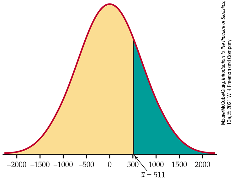
Figure 6.7 Comparison of the sample mean in Example 6.8 with the null hypothesized value 0.
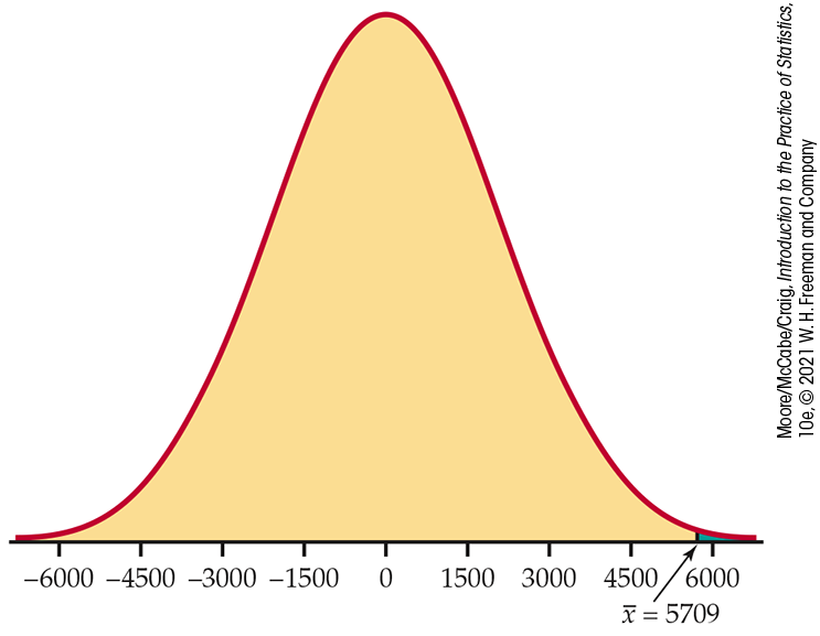
Figure 6.8 Comparison of the sample mean in Example 6.9 with the null hypothesized value 0.
Stating hypotheses
In Examples 6.8 and 6.9, we asked whether the difference in the observed means is reasonable if, in fact, there is no difference in the population means. To answer this, we begin by supposing that the statement following the “if” in the previous sentence is true. In other words, we suppose that the true difference is $0. We then ask whether the data provide evidence against the supposition we have made. If so, we have evidence in favor of an effect (the means are different) we are seeking. Often, the first step in a test of significance is to state a claim that we will try to find evidence against.
We abbreviate “null hypothesis” as
or, equivalently,
Note that the null hypothesis refers to the population means for all undergraduates, including those for whom we do not have data.
It is convenient also to give a name to the statement we hope or
suspect is true. This is called the
alternative
hypothesis
and is abbreviated as
or, equivalently,
![]() Hypotheses always refer to some populations or a model, not to a
particular outcome. For this reason, we must state
Hypotheses always refer to some populations or a model, not to a
particular outcome. For this reason, we must state
Because
The alternative hypothesis should express the hopes or suspicions we
bring to the data.
![]() It is cheating to first look at the data and then frame
It is cheating to first look at the data and then frame
Check-in
-
6.12 Dining court survey. During the summer, the dining court closest to your university residence was redesigned. A survey is planned to assess whether or not students think that the new design is an improvement. It will contain eight questions; a 7-point scale will be used for the answers, with scores less than 4 favoring the previous design and scores greater than 4 favoring the new design (to varying degrees). The average of the eight questions will be used as the student’s response. State the null and alternative hypotheses you would use for examining whether or not the new design is viewed more favorably.
-
6.13 DXA scanners. A dual-energy X-ray absorptiometry (DXA) scanner is used to measure bone mineral density for people who may be at risk for osteoporosis. One researcher believes that her scanner is not giving accurate readings. To assess this, the researcher uses an object called a “phantom” that has known mineral density
Test statistics
We will learn the form of significance tests in a number of common situations. Here are some principles that apply to most tests and that help in understanding these tests:
-
The test is based on a statistic that estimates the parameter that appears in the hypotheses. Usually, this is the same estimate we would use in a confidence interval for the parameter. When
-
Values of the estimate far from the hypothesized value give evidence against
-
To assess how far the estimate is from the hypothesized value, standardize the estimate. In many common situations the test statistic has the form
which refers to how many standard deviations the estimate is away from the hypothesized value of the parameter.
A test statistic measures compatibility between the null hypothesis and the data. We use it for the probability calculation that we need for our test of significance. It is a random variable with a distribution that we know.
Let’s return to our comparison of the grants and scholarship amount among planners and nonplanners and specify the hypotheses as well as calculate the test statistic.
Example 6.10 Average grants and scholarships amount of planners and nonplanners: The hypotheses.
In Example 6.8, the hypotheses are stated in terms of the difference in the average grants and scholarships amount between planners and nonplanners:
Because
We can also state the null hypothesis as
Example 6.11 Average grants and scholarships amount of planners and nonplanners: The test statistic.
In Example 6.8, the estimate of the difference is $511. Using methods that we will discuss in detail later, we can determine that the standard deviation of the estimate is $710. For this problem the test statistic is
For our data,
We have observed a sample estimate that is less than 1 standard deviation away from the hypothesized value of the parameter.
Because the sample sizes are sufficiently large for us to conclude that the distribution of the sample estimate is approximately Normal, the standardized test statistic z will have approximately the N(0, 1) distribution. We will use facts about the Normal distribution in what follows.
P-values
If all test statistics were Normal, we could base our conclusions on
the value of the z test statistic. In fact, the Supreme Court
of the United States has said that “two or three standard deviations”
“Extreme” means “far from what we would expect if
The key to calculating the P-value is knowing the sampling distribution of the test statistic. For the problems we consider in this chapter, we need only the standard Normal distribution for the test statistic z.
In
Example 6.8,
we want to know if the average grants and scholarships amount for
planners differs from the average grants and scholarships amount for
nonplanners. The difference we calculated based on our sample is $511,
which corresponds to 0.72 standard deviation away from zero—that is,
Example 6.12 Average grants and scholarships amount of planners and nonplanners: The P-value.
In Example 6.11, we found that the test statistic for testing
versus
is
If
The probability for being extreme in the negative direction is the same:
So the P-value is
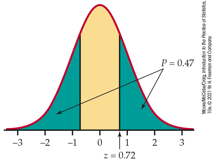
Figure 6.9 The
P-value,
Example 6.12. The P-value is the probability (when
This is the value that we reported on page 347. There is a 47% chance of observing a difference as extreme as the $511 in our sample if the true population difference is zero. This P-value tells us that our outcome is not particularly extreme. In other words, the data do not provide substantial evidence for us to doubt the validity of the null hypothesis.
Check-in
-
6.14 Normal curve and the P-value. A test statistic for a two-sided significance test for a population mean is
-
6.15 More on the Normal curve and the P-value. A test statistic for a two-sided significance test for a population mean is
Statistical significance
We started our discussion of the reasoning of significance tests
with the statement of null and alternative hypotheses. We then learned
that a test statistic is the tool used to examine the compatibility of
the observed data with the null hypothesis. Finally, we translated the
test statistic into a P-value to quantify the evidence against
We can compare the P-value we calculated with a fixed value
that we regard as decisive. This amounts to announcing in advance how
much evidence against
![]() “Significant” in the statistical sense does not mean
“important.”
The original meaning of the word is “signifying something.” In
statistics, significant is used to indicate only that the
evidence against the null hypothesis has reached the standard set by
“Significant” in the statistical sense does not mean
“important.”
The original meaning of the word is “signifying something.” In
statistics, significant is used to indicate only that the
evidence against the null hypothesis has reached the standard set by
Example 6.13 Average grants and scholarships amount of planners and nonplanners: The conclusion.
In Example 6.12, we found that the P-value is
There is an 47% chance of observing a difference as extreme as the
$511 in our sample if the true population difference is zero.
Because this P-value is larger than the
![]() This statement does not mean that we conclude that the null
hypothesis is true, only that the level of evidence we require to
reject the null hypothesis is not met.
Our criminal court system follows a similar procedure in which a
defendant is presumed innocent
This statement does not mean that we conclude that the null
hypothesis is true, only that the level of evidence we require to
reject the null hypothesis is not met.
Our criminal court system follows a similar procedure in which a
defendant is presumed innocent
If the P-value is small, we reject the null hypothesis. Here is the conclusion for our second example.
Example 6.14 Average amount paid for college by planner status: The conclusion.
In Example 6.9, we found that the difference in the average amount a family pays for college between planners and nonplanners was $5709. Because planners have access to more expensive options, we had a prior expectation that the planner average would be higher than the nonplanner average. It is appropriate to use a one-sided alternative in this situation. So, our hypotheses are
versus
The standard deviation is $1975 (again, we defer details regarding this calculation), and the test statistic is
Because only positive differences in parental contributions count against the null hypothesis, the one-sided alternative leads to the calculation of the P-value using the upper tail of the Normal distribution. The P-value is
The calculation is illustrated in
Figure 6.10. There is about a 2-in-1000 chance of observing a difference as
large as or larger than the $5709 in our sample if the true
population difference is zero. This P-value tells us that our
outcome is very rare. We conclude that the null hypothesis must be
false. Because the observed difference is positive, here is one way
to report the result: “The data clearly show that the average amount
a planning family pays for college is larger than the average amount
a nonplanning family pays for college
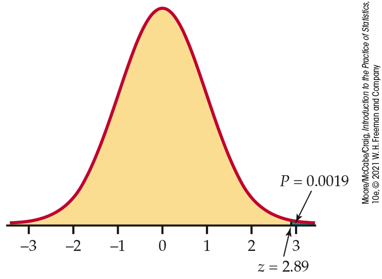
Figure 6.10 The
P-value,
Example 6.14. The P-value is the probability (when
Check-in
-
6.16 Finding significant z-scores. Consider a two-sided significance test for a population mean.
-
Sketch a Normal curve similar to that shown in Figure 6.9 (page 352) but find the value z such that
-
Based on your curve from part (a), what values of the z statistic are statistically significant at the
-
-
6.17 More on finding significant z-scores. Consider a one-sided significance test for a population mean, where the alternative is “greater than.”
-
Sketch a Normal curve similar to that shown in Figure 6.10 but find the value z such that
-
Based on your curve from part (a), what values of the z statistic are statistically significant at the
-
-
6.18 The Supreme Court speaks. The Supreme Court has said that z-scores beyond 2 or 3 are generally convincing statistical evidence. For a two-sided test, what significance level corresponds to
A test of significance is a process for assessing the significance of the evidence provided by data against a null hypothesis. The four steps common to all tests of significance are as follows:
-
State the null hypothesis
-
Calculate the value of the test statistic on which the test
will be based. This statistic usually measures how far the data are
from
-
Find the P-value for the observed data. This is the
probability, calculated assuming that
-
State a conclusion. One way to do this is to choose a
significance level
We will learn the details of many tests of significance in the following chapters. The proper test statistic is determined by the hypotheses and the data collection design. We use computer software or a calculator to find its numerical value and the P-value. The computer will not formulate your hypotheses for you, however. Nor will it decide if significance testing is appropriate or help you to interpret the P-value that it presents to you. These steps require judgment based on a sound understanding of this type of inference.
Tests for a population mean
![]()
Our discussion has focused on the reasoning of statistical tests, and we have outlined the key ideas for one type of procedure. Our examples focused on the comparison of two population means. Here is a summary for a test about one population mean.
We want to test the hypothesis that a parameter has a specified
value. This is the null hypothesis. For a test of a population mean
which often is expressed as
where
The test is based on data summarized as an estimate of the parameter.
For a population mean, this is the sample mean
Recall from
Chapter 5 that the
standard deviation of
Again from
Chapter 5 , if the
population is Normal, then
Suppose that we have calculated a test statistic
Similar reasoning applies when the alternative hypothesis states that
the true
We would make exactly the same calculation if we observed
Example 6.15 Percent energy from added sugars.

Dietary sugars can loosely be broken down into those naturally
occurring in foods and those that are added for taste or other
functional property. The added sugars, such as granulated sugar and
corn syrup, are typically associated with foods of poor nutrient
quality and are more strongly associated with obesity and diabetes.
One study used data from the National Health and Nutrition
Examination Survey (NHANES) to estimate the percent energy from
added sugars in various age categories. For the adult category
You decide to determine this percent for students at your large university. You survey 100 students and find the average to be 14.3%. Is there evidence that this mean percent differs from the reported adult mean?
The null hypothesis is “no difference” from the published mean
As usual in this chapter, we make the unrealistic assumption that
the population standard deviation is known. In this case, we’ll use
the standard deviation from the large national study,
We compute the test statistic:
Figure 6.11 illustrates the P-value, which is the probability that a standard Normal variable Z takes a value at least 1.05 away from zero. From Table A, we find that this probability is
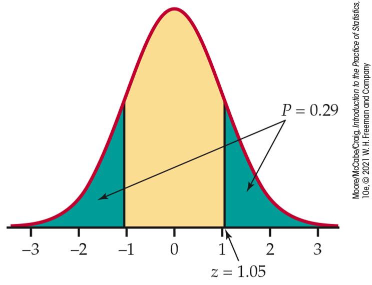
Figure 6.11 Sketch of
the P-value calculation for the two-sided test,
Example 6.15. The test statistic is
That is, if the population mean were 13.1%, almost 30% of the time
an SRS of size 100 would have a mean at least as far from 13.1% as
that of this sample. The observed
This z test result is valid provided that the 100 students in
the sample can be considered an SRS from the population of students at
your university and that
The data in
Example 6.15
do not establish that the mean
Tests of significance assess the evidence against
![]() Failing to find evidence against
Failing to find evidence against
Example 6.16 Significance test of the mean SATM score.
In a discussion of SAT Mathematics (SATM) scores, a friend comments,
“Because only California high school students considering college
take the SAT, the scores overestimate the mathematics ability of
typical high school seniors. I think that if all seniors took the
test, the mean score would be no more than 495.” You do not agree
with his claim and decide to use the SRS of 500 seniors from
Example 6.3
(page 331) to
assess the degree of evidence against it. Those 500 seniors had a
mean SATM score of
Because the claim states that the mean is “no more than 495,” the alternative hypothesis is one-sided. The hypotheses are
As we did in the discussion following
Example 6.3, we assume that
Because
Figure 6.12 illustrates this P-value. A mean score as large as that observed would occur roughly 12 times in 1000 samples if the population mean were 495. This is convincing evidence that the mean SATM score for all California high school seniors is higher than 495. You can confidently tell your friend that his claim is incorrect.
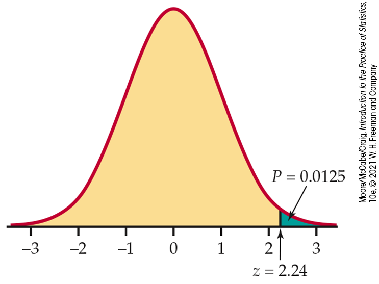
Figure 6.12 Sketch of
the P-value calculation for the one-sided test,
Example 6.16. The test statistic is
Check-in
-
6.19 Computing the test statistic and P-value. You will perform a significance test of
-
If
-
What is the P-value if
-
What is the P-value if
-
-
6.20 Testing a random number generator. Statistical software often has a “random number generator” that is supposed to produce numbers uniformly distributed between 0 and 1. If this is true, the numbers generated come from a population with
Two-sided significance tests and confidence intervals
Recall the basic idea of a confidence interval, discussed in
Section 6.1. We constructed an interval that would include the true value of
Example 6.17 Water quality testing.
![]()

The Deely Laboratory is a drinking-water testing and analysis
service. One of the common contaminants it tests for is lead. Lead
enters drinking water through corrosion of plumbing materials, such
as lead pipes, fixtures, and solder. The service knows that its
analysis procedure is unbiased but not perfectly precise, so the
laboratory analyzes each water sample three times and reports the
mean result. The repeated measurements follow a Normal distribution
quite closely. The standard deviation of this distribution is a
property of the analytic procedure and is known to be
The Deely Laboratory has been asked by a university to evaluate a
claim that the drinking water in the Student Union has a lead
concentration above the Environmental Protection Agency’s (EPA’s)
action level of 15 ppb. Because the true concentration of the sample
is the mean
We use the two-sided alternative here because there is no prior
evidence to substantiate a one-sided alternative. The lab chooses
the 1% level of significance,
Three analyses of one specimen give concentrations
The sample mean of these readings is
The test statistic is
Because the alternative is two-sided, the P-value is
We cannot find this probability in
Table A. The largest value of z in that table is 3.49. All that we
can say from
Table A
is that P is less than
We can compute a 99% confidence interval for the same data to get a
likely range for the actual mean concentration
Example 6.18 99% confidence interval for the mean concentration.
![]()
The 99% confidence interval for
The hypothesized value
at the 1% significance level. On the other hand, we cannot reject
at the 1% level in favor of the two-sided alternative
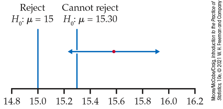
Figure 6.13 The link
between two-sided significance tests and confidence intervals. For
the study described in
Examples 6.17
and
6.18,
values of
The calculation in
Example 6.17
for a 1% significance test is very similar to the calculation for a
99% confidence interval. In fact, a two-sided test at significance
level
Check-in
-
6.21 Two-sided significance tests and confidence intervals. The P-value for a two-sided significance test with null hypothesis
-
Does the 95% confidence interval include the value 30? Explain.
-
Does the 99% confidence interval include the value 30? Explain.
-
-
6.22 More on two-sided significance tests and confidence intervals. A 95% confidence interval for a population mean is (29, 58).
-
Can you reject the null hypothesis that
-
Can you reject the null hypothesis that
-
The P-value versus a statement of significance
The observed result in
Example 6.17
was
gives a better sense of how strong the evidence is.
The P-value is the smallest level
Example 6.19 Test of the mean SATM score: Significance.
In Example 6.16, we tested the hypotheses
concerning the mean SAT Mathematics score
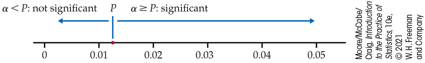
Figure 6.14 Link
between the P-value and the significance level
A P-value is more informative than a reject-or-not finding at a
fixed significance level. But assessing significance at a fixed-level
Example 6.20 Average grants and scholarships amount of planners and nonplanners: Assessing significance.
In
Example 6.11
(page 351), we
found the test statistic
Check-in
-
6.23 P-value and the significance level. The P-value for a significance test is 0.033.
-
Do you reject the null hypothesis at level
-
Do you reject the null hypothesis at level
-
Explain how you determined your answers to parts (a) and (b).
-
-
6.24 More on P-value and the significance level. The P-value for a significance test is 0.069.
-
Do you reject the null hypothesis at level
-
Do you reject the null hypothesis at level
-
Explain how you determined your answers to parts (a) and (b).
-
-
6.25 One-sided and two-sided P-values. The P-value for a two-sided significance test is 0.084.
-
State the P-values for the two one-sided tests.
-
What additional information do you need to properly assign these P-values to the
-
Section 6.2 SUMMARY
-
A test of significance is intended to assess the evidence provided by data against a null hypothesis
-
The hypotheses are stated in terms of population parameters. Usually
-
The test is based on a test statistic. The P-value is the probability, computed assuming that
-
If the P-value is as small as or smaller than a specified value
-
Significance tests for the hypothesis
This test assumes that the sample is an SRS of size n and either a Normal population or a large enough sample size n. P-values are computed from the Normal distribution (Table A). Fixed
Section 6.2 EXERCISES
-
6.26 What’s wrong? For each of the following statements, explain what is wrong and why.
-
A researcher tests the following null hypothesis:
-
A random sample of size 30 is taken from a population that is assumed to have a standard deviation of 5. The standard deviation of the sample mean is 5/30.
-
A study with
-
A researcher tests the hypothesis
-
-
6.27 What’s wrong? For each of the following statements, explain what is wrong and why.
-
A significance test rejected the null hypothesis that the sample mean is equal to 500.
-
A test preparation company wants to test that the average score of its students on the ACT is better than the national average score of 21.2. The company states its null hypothesis to be
-
A study summary says that the results are statistically significant with
-
The z test statistic is equal to 0.018. Because this is less than
-
-
6.28 Determining hypotheses. State the appropriate null hypothesis
-
A 2019 study reported that 97.8% of college students own a cell phone. You plan to take an SRS of college students to see if the percent has increased.
-
The examinations in a large freshman chemistry class are scaled after grading so that the mean score is 75. The professor thinks that students who do not attend their recitation section will have a lower mean score than the class as a whole. This semester’s students who do not attend their recitation can be considered a sample from the population of all students who would not attend, so she compares their mean score with 75.
-
The student newspaper at your college recently changed the format of its opinion page. You want to test whether students find the change an improvement. You take a random sample of students who regularly read the newspaper. They are asked to indicate their opinions on the changes using a five-point scale:
-
-
6.29 More on determining hypotheses. State the null hypothesis
-
A university gives credit in first-year calculus to students who pass a placement test. The mathematics department wants to know if students who get credit in this way differ in their success with second-year calculus. Scores in second-year calculus are scaled so the average each year is equivalent to a 77. This year, 21 students who took second-year calculus passed the placement test.
-
Experiments on learning in animals sometimes measure how long it takes a mouse to find its way through a maze. The mean time is 20 seconds for one particular maze. A researcher thinks that playing rap music will cause the mice to complete the maze more slowly. She measures how long each of 12 mice takes with the rap music as a stimulus.
-
The average square footage of one-bedroom apartments in a new student-housing development is advertised to be 880 square feet. A student group thinks that the apartments are smaller than advertised. They hire an engineer to measure a sample of apartments to test their suspicion.
-
-
6.30 Even more on determining hypotheses. In each of the following situations, state an appropriate null hypothesis
-
A sociologist asks a large sample of high school students which television channel they like best. She suspects that a higher percent of males than of females will name MTV as their favorite channel.
-
An education researcher randomly divides sixth-grade students into two groups for physical education class. He teaches both groups basketball skills, using the same methods of instruction in both classes. He encourages Group A with compliments and other positive behavior but acts cool and neutral toward Group B. He hopes to show that positive teacher attitudes result in a higher mean score on a test of basketball skills than do neutral attitudes.
-
An education researcher believes that, among college students, there is a negative correlation between time spent at social network sites and self-esteem, measured on a scale of 0–100. To test this, she gathers social-networking information and self-esteem data from a sample of students at your college.
-
-
6.31 Translating research questions into hypotheses. Translate each of the following research questions into appropriate
-
U.S. Census Bureau data show that the mean household income in the area served by a shopping mall is $78,800 per year. A market research firm questions shoppers at the mall to find out whether the mean household income of mall shoppers is higher than that of the general population.
-
Last year, your online registration technicians took an average of 0.4 hour to respond to trouble calls from students trying to register. Do this year’s data show a different average response time?
-
In 2019, Netflix’s vice president of original content stated that the average Netflix subscriber spends two hours a day on the service.15 Because of an increase in competing services, you believe this average has declined this year.
-
-
6.32 Computing the P-value. A test of the null hypothesis
-
What is the P-value if the alternative is
-
What is the P-value if the alternative is
-
What is the P-value if the alternative is
-
-
6.33 More on computing the P-value. A test of the null hypothesis
-
What is the P-value if the alternative is
-
What is the P-value if the alternative is
-
What is the P-value if the alternative is
-
-
6.34 Consumption of neurotoxic insecticide delays migration. Some Canadian researchers recently investigated the impact of songbirds consuming a widely used insecticide.16 They reported that white-crowned sparrows fed 1.2 mg/kg body mass of imidacloprid had an average mass loss of 3%
-
6.35 Average starting salary, continued. Refer to Exercise 6.12 (page 345). Use the information presented in the exercise to test whether the average income of graduates from your institution is different from the national average
-
6.36 Change in consumption of sweet snacks? Refer to Exercise 6.13 (page 345). A similar study performed four years earlier reported the average consumption of sweet snacks among healthy-weight children aged 12 to 19 years to be 369.4 kilocalaries per day (kcal/d). Does this current study suggest a change in the average consumption? Perform a significance test using the 5% significance level. Write a short paragraph summarizing the results.
-
6.37 Peer pressure and choice of major. A study followed a cohort of students entering a business/economics program.17 All students followed a common track during the first three semesters and then chose to specialize in either business or economics. Through a series of surveys, the researchers were able to classify roughly 50% of the students as either peer driven (ignored abilities and chose major to follow peers) or ability driven (ignored peers and chose major based on ability). When looking at entry wages after graduation, the researchers conclude that a peer-driven student can expect an average wage that is 13% less than that of an ability-driven student. The report states that the significance level is
-
6.38 Symbol of wealth in ancient China? Every society has its own symbols of wealth and prestige. In ancient China, it appears that owning pigs was such a symbol. Evidence comes from examining burial sites. If the skulls of sacrificed pigs tend to appear along with expensive ornaments, that suggests that the pigs, like the ornaments, signal the wealth and prestige of the person buried. A study of burials from around 3500 b.c. concluded that “there are striking differences in grave goods between burials with pig skulls and burials without them . . .. A test indicates that the two samples of total artifacts are significantly different at the 0.01 level.”18 Explain clearly why “significantly different at the 0.01 level” gives good reason to think that there really is a systematic difference between burials that contain pig skulls and those that lack them.
-
6.39 Alcohol awareness among college students. A study of alcohol awareness among college students reported a higher awareness for students enrolled in a health and safety class than for those enrolled in a statistics class.19 The difference is described as being statistically significant. Explain what this means in simple terms and offer an explanation for why the health and safety students had a higher mean score.
-
 6.40 Are the pine trees randomly distributed from north to
south?
In
Example 6.1
(page 329),
we looked at the distribution of longleaf pine trees in the Wade
Tract. One way to formulate hypotheses about whether or not the
trees are randomly distributed in the tract is to examine the
average location in the north–south direction. The values range
from 0 to 200, so if the trees are uniformly distributed in this
direction, any difference from the middle value (100) should be
due to chance variation. The sample mean for the 584 trees in
the tract is 99.74. A theoretical calculation based on the
assumption that the trees are uniformly distributed gives a
standard deviation of 58. Carefully state the null and
alternative hypotheses in terms of this variable. Note that this
requires that you translate the research question about the
random distribution of the trees into specific statements about
the mean of a probability distribution. Test your hypotheses,
report your results, and write a short summary of what you have
found.
6.40 Are the pine trees randomly distributed from north to
south?
In
Example 6.1
(page 329),
we looked at the distribution of longleaf pine trees in the Wade
Tract. One way to formulate hypotheses about whether or not the
trees are randomly distributed in the tract is to examine the
average location in the north–south direction. The values range
from 0 to 200, so if the trees are uniformly distributed in this
direction, any difference from the middle value (100) should be
due to chance variation. The sample mean for the 584 trees in
the tract is 99.74. A theoretical calculation based on the
assumption that the trees are uniformly distributed gives a
standard deviation of 58. Carefully state the null and
alternative hypotheses in terms of this variable. Note that this
requires that you translate the research question about the
random distribution of the trees into specific statements about
the mean of a probability distribution. Test your hypotheses,
report your results, and write a short summary of what you have
found.
-
6.41 Are the pine trees randomly distributed from east to
west?
Answer the questions in the previous exercise for the east–west
direction, for which the sample mean is 113.8.
-
6.42 Who is the author? Statistics can help decide the authorship of literary works. Sonnets by a certain Elizabethan poet are known to contain an average of
Give the z test statistic and its P-value. What do you conclude about the authorship of the new poems?
-
6.43 Attitudes toward school. The Survey of Study Habits and Attitudes (SSHA) is a psychological test that measures the motivation, attitude toward school, and study habits of students. Each scores ranges from 0 to 200. The mean attitude score for U.S. college students is about 110, and the standard deviation is about 25. A teacher who suspects that older students have better attitudes toward school gives the SSHA to 25 students who are at least 30 years of age. Their mean score is
-
Assuming that
Report the P-value of your test and state your conclusion clearly.
-
Your test in part (a) required two important assumptions in addition to the assumption that the value of
-
-
6.44 Nutritional intake among Canadian high-performance athletes. Since previous studies have reported that elite athletes are often deficient in their nutritional intake (for example, total calories, carbohydrates, protein), a group of researchers decided to evaluate Canadian high-performance athletes.20 A total of
-
State the appropriate
-
Assuming a standard deviation of 880 kcal/d, carry out the test. Give the P-value, and then interpret the result in plain language.
-
-
6.45 Fuel economy. In 2017, the Environmental Protection Agency (EPA) changed how it calculates window-sticker gas mileage. For many models, this meant a

25.9 25.4 24.7 26.1 24.7 25.7 25.2 26.2 26.1 25.3 24.3 24.6 26.5 25.8 25.8 25.6 The average combined mpg for the 2017 Toyota RAV4 LE was 26.0 mpg. Using
-
 6.46 Impact of
-
6.47 Effect of changing
-
6.48 Changing to a two-sided alternative.
Repeat the previous exercise but with the two-sided alternative
hypothesis. How does this change affect which values of
-
6.49 Changing the sample size.
Refer to
Exercise 6.46. Suppose that you increase the sample size n from 10 to
100. Again, make a table giving
-
6.50 Impact of
-
6.51 Changing to a two-sided alternative, continued.
Repeat the previous exercise but with the two-sided alternative
hypothesis. How does this change affect the P-values
associated with each
-
6.52 Other changes and the P-value.
Refer to the previous exercise.
-
What happens to the P-values when you change the significance level
-
What happens to the P-values when you change the sample size n from 10 to 100? Explain the result.
-
-
6.53 Understanding levels of significance. Explain in plain language why a significance test that is significant at the 1% level must always be significant at the 5% level.
-
6.54 More on understanding levels of significance. You are told that a significance test is significant at the 5% level. From this information, can you determine whether or not it is significant at the 1% level? Explain your answer.
-
6.55 Test statistic and levels of significance. Consider a significance test for a null hypothesis versus a two-sided alternative. Give a value of z that will give a result significant at the 1% level but not at the 0.5% level.
-
6.56 Using Table D to find a P-value. You have performed a two-sided test of significance and obtained a value of
-
6.57 More on using Table D to find a P-value. You have performed a one-sided test of significance and obtained a value of
-
6.58 Using Table A and Table D to find a P-value. Consider a significance test for a null hypothesis versus a two-sided alternative. Between what values from Table D does the P-value for an outcome
-
6.59 More on using Table A and Table D to find a P-value. Refer to the previous exercise. Find the P-value for