9.2 Goodness of Fit in Chapter 9 Inference for Categorical Data

9.2 Goodness of Fit

Data set icon for Vtm.

In Section 9.1, we discussed the use of the chi-square test to compare categorical-variable distributions of c populations. We now consider a slight variation on this scenario where we compare a sample from one population with a hypothesized distribution. Here is an example that illustrates the basic ideas.

Example 9.14 Sampling in the Adequate Calcium Today (ACT) study.

The ACT study was designed to examine relationships among bone growth patterns, bone development, and calcium intake. Participants were more than 14,000 adolescents from six states: Arizona (AZ), California (CA), Hawaii (HI), Indiana (IN), Nevada (NV), and Ohio (OH). After the major goals of the study were completed, the investigators decided to do an additional analysis of the written comments made by the participants during the study.

Because the number of participants was so large, a sampling plan was devised to select sheets containing the written comments of approximately 10% of the participants. A systematic sample (see page 191) of every 10th comment sheet was retrieved from each storage container for analysis.⁸ Here are the counts for each of the six states:

Number of study participants in the sample
AZ	CA	HI	IN	NV	OH	Total
167	257	257	297	107	482	1567

There were 1567 study participants in this sample. Did it result in a representative sample from the collection of all participants? One way to answer this is to use the proportions of students from each of the states in the original sample of more than 14,000 participants as the population values.⁹ Here are the proportions:

Population proportions
AZ	CA	HI	IN	NV	OH	Total
0.105	0.172	0.164	0.188	0.070	0.301	100.000

Let’s see how well our sample reflects the state population proportions. We start by computing expected counts. Because 10.5% of the population is from Arizona, we expect the sample to have about 10.5% from Arizona. Therefore, because the sample has 1567 subjects, our expected count for Arizona is

expected count for Arizona=0.105(1567)=164.535

Here are the expected counts for all six states:

Expected counts
AZ	CA	HI	IN	NV	OH	Total
164.54	269.52	256.99	294.60	109.69	471.67	1567.01

Check-in

9.15 Why is the sum 1567.01? Refer to the table of expected counts in Example 9.14. Explain why the sum of the expected counts is 1567.01 and not 1567.
9.16 Calculate the expected counts. Refer to Example 9.14. Find the expected counts for the other five states. Report your results with three places after the decimal, as we did for Arizona. When you sum using three decimal places, does the rounding error go away?

As we saw with the expected counts in the analysis of two-way tables in Section 9.1, we do not really expect the observed counts to be exactly equal to the expected counts. Different samples under the same conditions would give different counts. We expect the average of these counts to be equal to the expected counts when the null hypothesis is true. How close do we think the counts and the expected counts should be?

We can think of our table of observed counts in Example 9.14 as a one-way table with six cells, each with a count of the number of subjects sampled from a particular state. Our question of interest is translated into a null hypothesis that says that the observed proportions of students in the six states can be viewed as random samples from the subjects in the ACT study. The alternative hypothesis is that the process generating the observed counts, a form of systematic sampling in this case, does not provide samples that are compatible with this hypothesis. In other words, the alternative hypothesis says that there is some bias in the way we selected the subjects whose comments we will examine.

Our analysis of these data is very similar to the analyses of two-way tables that we studied in Section 9.1. We have already computed the expected counts. We now construct a chi-square statistic that measures how far the observed counts are from the expected counts. Here is a summary of the procedure.

The chi-square goodness-of-fit test

Data for n observations of a categorical variable with k possible outcomes are summarized as observed counts, n1,n2,…,nk, in k cells. The null hypothesis specifies probabilities p1,p2,…,pk for the possible outcomes. The alternative hypothesis says that the true probabilities of the possible outcomes are not the probabilities specified in the null hypothesis.

For each cell, multiply the total number of observations n by the specified probability to determine the expected counts:

expected count=npi

The chi-square statistic measures how much the observed cell counts differ from the expected cell counts. The formula for the statistic is

X2=∑=(observed count-expected count)2expected count

The degrees of freedom are k-1, and P-values are computed from the chi-square distribution.

Use this procedure when the expected counts are all 5 or more.

Example 9.15 The goodness-of-fit test for the ACT study.

For Arizona, the observed count is 167. In Example 9.14, we calculated the expected count, 164.535. The contribution to the chi-square statistic for Arizona is

(observed count-expected count)2expected count=(167−164.535)2164.535=0.0369

We use the same approach to find the contributions to the chi-square statistic for the other five states. The expected counts are all at least 5, so we can proceed with the significance test.

The sum of these six values is the chi-square statistic,

X2=0.93

The degrees of freedom are the number of cells minus 1, df=6−1=5. We calculate the P-value using Table F or software. From Table F, we can determine P>0.25. We conclude that the observed counts are compatible with the hypothesized proportions. The data do not provide any evidence that our systematic sample was biased with respect to selection of subjects from different states.

Check-in

9.17 Compute the chi-square statistic. For each of the other five states, compute the contribution to the chi-square statistic using the method illustrated for Arizona in Example 9.15. (You can use the expected counts that you found in Check-in question 9.16 for these calculations.) Show that the sum of these values is the chi-square statistic.

Example 9.16 The goodness-of-fit test from software.

Data set icon for act.

Software output from Minitab, SPSS, and JMP for this problem is given in Figure 9.10. Minitab and SPSS report the P-value as 0.968. JMP gives an additional place after the decimal, 0.9679. Note that the SPSS output includes a column titled “Residual.” For tables of counts, a residual for a cell is defined as

residual=observed count - expected countexpected count

The chi-square statistic is the sum of the squares of these residuals. Note that the residual reported by SPSS is the numerator of this ratio.

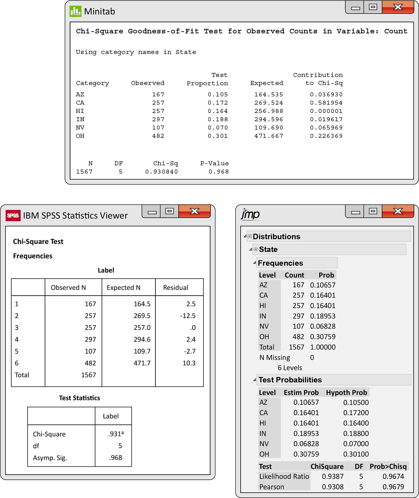
Minitab, SPSS, and JMP outputs for goodness of fit. — Figure 9.10 Minitab, SPSS, and JMP outputs, Example 9.16.

The Minitab output is titled, chi square goodness of fit test for observed counts in variable, count. Using category names in state. Two tables are shown with the following data. First table. Category, A Z. Observed, 167. Test proportion, 0.105. Expected, 164.535. Contribution to chi square, 0.036930. Category, C A. Observed, 257. Test proportion, 0.172. Expected, 269.524. Contribution to chi square, 0.581954. Category, H I. Observed, 257. Test proportion, 0.164. Expected, 256.988. Contribution to chi square, 0.000001. Category, I N. Observed, 297. Test proportion, 0.188. Expected, 294.596. Contribution to chi square, 0.19617. Category, N V. Observed, 107. Test proportion, 0.070. Expected, 109.690. Contribution to chi square, 0.65969. Category, O H. Observed, 482. Test proportion, 0.301. Expected, 471.667. Contribution to chi square, 0.226369. Second table. N, 1567. D F, 5. Chi square, 0.930840. P value, 0.968. The SPSS output is titled chi square, frequencies. It shows two tables with the following data. First table. Label. Level, 1. Observed N, 167. Expected N, 164.5. Residual, 2.5. Level, 2. Observed N, 257. Expected N, 269.5. Residual, negative 12.5. Level, 3. Observed N, 257. Expected N, 257.0. Residual, 0.0. Level, 4. Observed N, 297. Expected N, 294.6. Residual, 2.4. Level, 5. Observed N, 107. Expected N, 109.7. Residual, negative 2.7. Level, 6. Observed N, 482. Expected N, 471.7. Residua 10.3. Total observed N, 1567. Second table. test statistics. Chi square, 0.931. d f, 5. Asymptotic significance, 0.968. The JMP output shows three expanded dropdown list menus, distributions, state, frequencies. A table shows the following data. Level, A Z. Count, 167. Probability, 0.10657. Level, C A. Count, 257. Probability, 0.16401. Level, H I. Count, 257. Probability, 0.16401. Level, I N. Count, 297. Probability, 0.18953. Level, N V. Count, 107. Probability, 0.06828. Level, O H. Count, 482. Probability, 0.30759. Level, total. Count, 1567. Probability, 1.0000. N missing, 0. Another expanded menu, test probabilities, shows two tables with the following data. First table. Level, A Z. Estimated probability, 0.10657. Hypothetical probability, 0.10500. Level, C A. Estimated probability, 0.16401. Hypothetical probability, 0.17200. Level, H I. Estimated probability, 0.16401. Hypothetical probability, 0.16400. Level, I N. Estimated probability, 0.18953. Hypothetical probability, 0.18800. Level, N V. Estimated probability, 0.06828. Hypothetical probability, 0.07000. Level, O H. Estimated probability, 0.30759. Hypothetical probability, 0.30100. Second table. Test, likelihood ratio. Chi square, 0.9387. D F, 5. Probability greater than chi square. 0.9674. Test, Pearson. Chi square, 0.9308. D F, 5. Probability greater than chi square, 0.9679.

Some software packages do not provide routines for computing the chi-square goodness-of-fit test. However, a very simple trick can be used to produce the results from software that can analyze two-way tables. Make a two-way table in which the first column contains k cells with the observed counts. Add a second column with counts that correspond exactly to the probabilities specified by the null hypothesis, with a very large number of observations. Then perform the chi-square significance test for two-way tables.

Check-in

9.18 Distribution of M&M colors. M&M Mars Company has varied the mix of colors for M&M’s Plain Chocolate Candies over the years. These changes in color blends are made based on the results of consumer preference tests. Recently, the color distribution was reported to be 13% brown, 14% yellow, 13% red, 20% orange, 24% blue, and 16% green.¹⁰ You open up a 14-ounce bag of M&M’s and find 61 brown, 59 yellow, 49 red, 77 orange, 141 blue, and 88 green. Use a goodness-of-fit test to examine how well this bag fits the percents stated by M&M Mars Company.

Example 9.17 The sign test as a goodness-of-fit test.

A study of the effect of the full moon on aggressive behaviors of dementia patients included 15 patients, 14 of whom exhibited a greater number of aggressive behaviors on full moon days than on other days. The sign test (page 401) tests the null hypothesis that patients are equally likely to exhibit more aggressive behaviors on full moon days and on other days. Because n=15, the sample proportion is p^=14/15, and the null hypothesis is H0: p=0.5.

To look at these data from the viewpoint of goodness of fit, we think of the data as two counts: patients who had a greater number of aggressive behaviors on full moon days and patients who had a greater number of aggressive behaviors on other days.

Counts
Moon	Other	Total
14	1	15

If the two outcomes are equally likely, the expected counts are both 7.5 (15×0.5). The expected counts are both greater than 5, so we can proceed with the significance test.

The test statistic is

X2=(14−7.5)27.5+(1−7.5)27.5=5.633+5.633=11.27

We have k=2, so the degrees of freedom are 1. From Table F, we conclude that P<0.001.

The sign test can test the null hypothesis versus the one-sided alternative that there was a “moon effect.” Within the framework of the goodness-of-fit test, we test only the general alternative hypothesis that the distribution of the counts do not follow the specified probabilities. Note that the P-value for the sign test versus the one-sided alternative is 0.000488, approximately one-half of the value that we reported from Table F in Example 9.17.

Section 9.2 SUMMARY

The chi-square goodness-of-fit test is used to compare the sample distribution of a categorical variable from a population with a hypothesized distribution. The data for n observations with k possible outcomes are summarized as observed counts, n1,n2,…,nk, in k cells. The null hypothesis specifies probabilities p1,p2,…,pk for the possible outcomes.
The analysis of these data is similar to the analyses of two-way tables discussed in Section 9.1. For each cell, the expected count is determined by multiplying the total number of observations n by the specified probability pi. The null hypothesis is tested by the usual chi-square statistic, which compares the observed counts, ni, with the expected counts. Under the null hypothesis, X2 has approximately the χ2 distribution with df=k−1.

Now that you have completed this section, you will be able to:

Compute expected counts, given a sample size and the probabilities specified by a null hypothesis for a chi-square goodness-of-fit test. Review Example 9.14 (page 505) and try Exercise 9.15.
Find the chi-square test statistic and its P-value. Review Example 9.15 (page 507) and try Exercise 9.17.
Interpret the results of a chi-square goodness-of-fit significance test. Review Example 9.15 (page 507) and try Exercise 9.19.

Section 9.2 EXERCISES

9.14 What’s wrong? Each of the following statements contains an error. Describe each error and explain why the statement is wrong.
1. A goodness-of-fit test can be used to compare the observed distribution of a categorical variable with a distribution specified by an alternative hypothesis.
2. The residuals for a chi-square goodness-of-fit test are all positive.
3. The expected counts for a goodness-of-fit test are computed by multiplying the sample size by the sample proportion.
9.15 Is the coin fair? In Example 4.3 (page 207), we learned that the South African statistician John Kerrich tossed a coin 10,000 times while imprisoned by the Germans during World War II. The coin came up heads 5067 times.
1. Formulate the question about whether or not the coin was fair as a goodness-of-fit hypothesis.
2. Compute the expected counts and explain what they tell us.
9.16 Goodness of fit to a standard Normal distribution. Computer software generated 300 random numbers that should look as if they are from the standard Normal distribution. They are categorized into five groups: (1) less than or equal to −0.7, (2) greater than −0.7 and less than or equal to −0.3, (3) greater than −0.3 and less than or equal to 0.3, (4) greater than 0.3 and less than or equal to 0.7, and (5) greater than 0.7. The counts in the five groups are 73, 39, 82, 49, and 57, respectively. Find the probabilities for these five intervals using Table A. Then compute the expected number for each interval for a sample of 300. Finally, perform the goodness-of-fit test and summarize your results.
9.17 Test the hypothesis that the coin fair. Refer to Exercise 9.15. Find the chi-square statistic and the P-value.
9.18 More on the goodness of fit to a standard Normal distribution. Refer to Exercise 9.16. Use software to generate a sample of 300 Normal random variables with mean 10 and standard deviation 5. Choose a set of intervals and perform the goodness-of-fit test.
9.19 Interpret the results of the coin tossing analysis. Refer to Exercises 9.15 and 9.17. Write a short summary of your analysis of John Kerrich’s coin tossing, including the results of the chi-square test.
9.20 Goodness of fit to a Poisson distribution. Refer to Example 5.30 (page 316), where a Poisson distribution is described as a model for the number of Wi-Fi slowdowns per day. The mean number of slowdowns is 3.7. In this setting, the probability for 0, 1, or 2 slowdowns is 0.28543, the probability for 4, 5, or 6 slowdowns is 0.54466, and the probability for 7 or more slowdowns is 0.16991. Suppose that you record the number of slowdowns for the next 100 days. Your observed counts of slowdowns are 27 for 0, 1, or 2 slowdowns, 56 for 4, 5, or 6 slowdowns, and 17 for 7 or more slowdowns. Use these data to test the hypothesis that slowdowns are distributed according to this Poisson distribution.
9.21 More on the goodness of fit to a Poisson distribution. Refer to the previous exercise. Repeat the analysis using 41, 35, and 24 as the observed counts. What do you conclude?