Chapter 12 EXERCISES
-
12.36 What’s wrong? For each of the following, explain what is wrong and why.
-
In rejecting the null hypothesis, one can conclude that all the means are different from one another.
-
A multiple-comparisons procedure is used to compare a relationship among means that was specified prior to looking at the data.
-
The ANOVA F statistic will be large when the within-group variation is much larger than the between-group variation.
-
The Bonferroni method will find at least as many pairs of means different as the LSD method.
-
-
12.37 Organic foods and morals? Organic foods are often marketed using moral terms such as “honesty” and “purity.” Is this just a marketing strategy, or is there a conceptual link between organic food and morality? In one experiment, 62 undergraduates were each randomly assigned to one of three food conditions (organic, comfort, and control).13 First, each participant was given a packet of four food types from the assigned condition and told to rate the desirability of each food on a seven-point scale. Then, each was presented with a list of six moral transgressions and asked to rate each on a seven-point scale ranging from

-
Make a table giving the sample size, mean, and standard deviation for each group. Is it reasonable to pool the variances?
-
Generate a histogram for each of the groups. Can we feel confident that the sample means are approximately Normal? Explain your answer.
-
-
12.38 Organic foods and morals (continued). Refer to the previous exercise.
-
Analyze the scores using one-way ANOVA. Report the test statistic, degrees of freedom, and P-value.
-
Assess the assumptions necessary for inference by examining the residuals. Summarize your findings. Do they agree with your conclusions in the previous exercise?
-
Compare the groups using the least-significant differences method.
-
A higher score is associated with a harsher moral judgment. Using the results from parts (a) and (c), write a short summary of your conclusions.
-
-
12.39 Organic foods and friendly behavior? Refer to Exercise 12.37 for the design of the experiment. After rating the moral transgressions, the participants were told that “another professor from another department is also conducting research and really needs volunteers.” They were also told that they would not receive compensation or course credit for their help and then were asked to write down the number of minutes (out of 30) that they would be willing to volunteer. This sort of question is often used to measure a person’s prosocial behavior.
-
Figure 12.17 contains the Excel output for the analysis of this response variable. Write a one-paragraph summary of your conclusions.
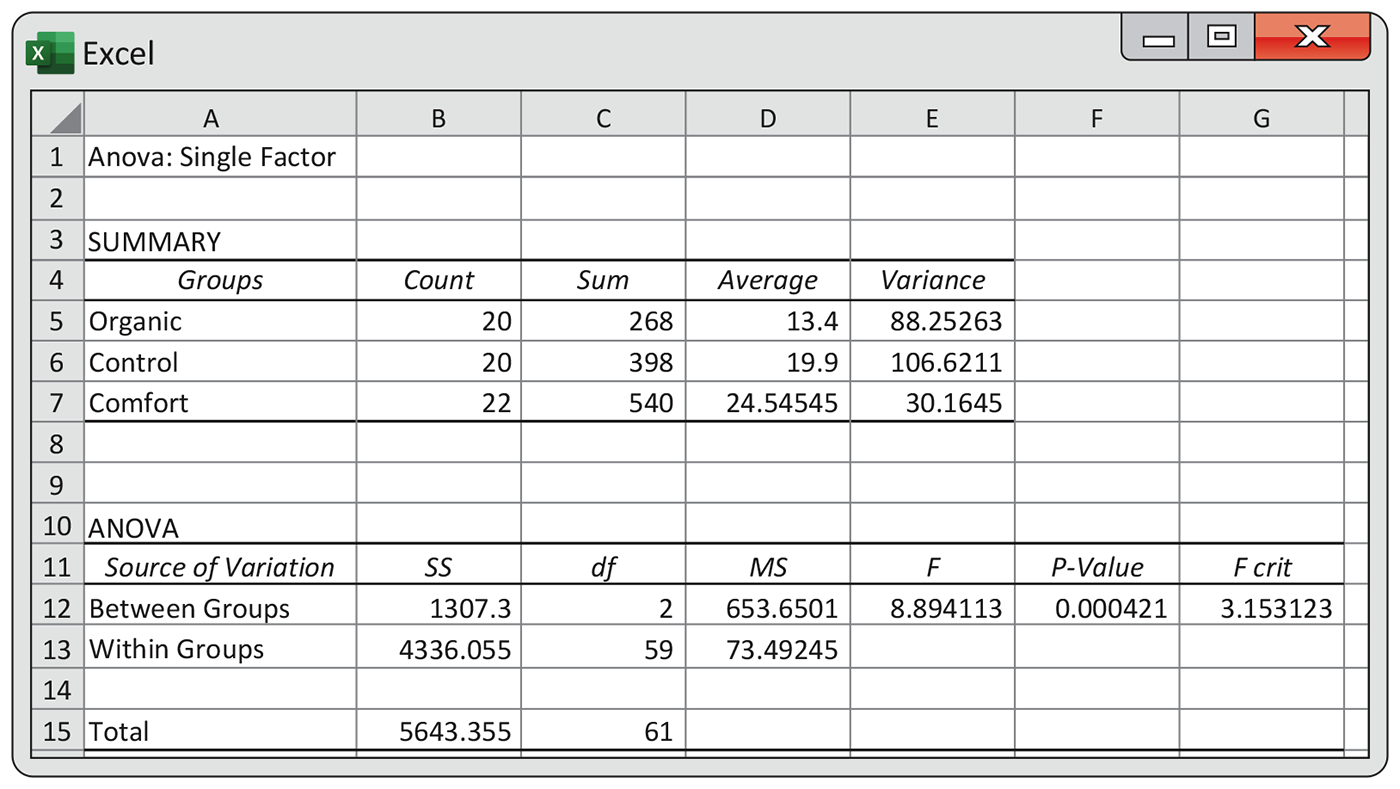
Figure 12.17 Excel one-way ANOVA output, Exercise 12.39.
- Figure 12.18 contains a residual plot and a Normal quantile plot of the residuals. Are there any concerns regarding the assumptions necessary for inference? Explain your answer.
-
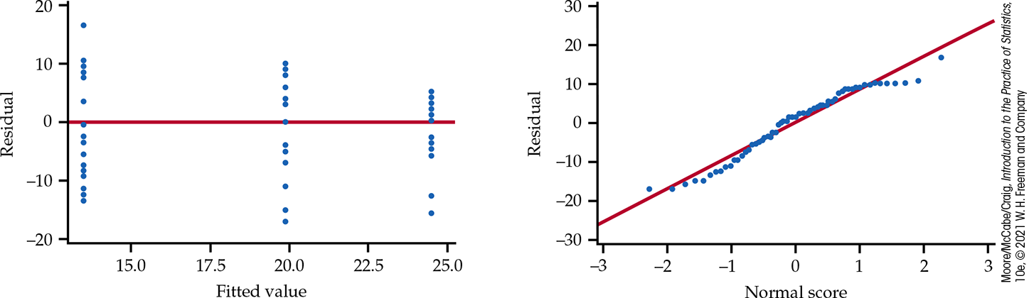
Figure 12.18 Residual plot and Normal quantile plot, Exercise 12.39.
-
-
 12.40 The effect of increased variation within groups.
The One-Way ANOVA applet lets you see how the
F statistic and the P-value depend on the
variability of the data within groups, the sample size, and the
differences among the means.
12.40 The effect of increased variation within groups.
The One-Way ANOVA applet lets you see how the
F statistic and the P-value depend on the
variability of the data within groups, the sample size, and the
differences among the means.
-
The graph shows the means of the three groups. Move these up and down until you get a configuration that gives a P-value of about 0.01. What is the value of the F statistic?
-
Now increase the variation within the groups by increasing the standard deviation. Describe what happens to the F statistic and the P-value.
-
Using between- and within-group variation, explain why the F statistic and P-value change in this way.
-
-
12.41 The effect of increased variation between groups.
Set the common standard deviation for the
One-Way ANOVA applet at a middle value. Set the means of
the three groups so that they are approximately equal.
-
What is the F statistic? Give its P-value.
-
Move the mean of the second group up and the mean of the third group down. Describe the effect on the F statistic and its P-value. Explain why they change in this way.
-
-
12.42 The effect of increased sample size. Set
the common standard deviation for the One-Way ANOVA applet
at a middle value and set the means to roughly 5.00, 4.50, and
5.25, respectively.
-
What are the F statistic, its degrees of freedom, and the P-value?
-
Slide the sample size bar to the right so
-
Explain why the F statistic and P-value change in this way as n increases.
-
-
12.43 Innovative wine packaging. Are wine bottles outdated? A group of researchers randomly assigned 247 German consumers to one of three wine packaging styles. They were a bottle with a screw cap (SC), a wine bag-in-box (BiB), and a four-pack of single-serving StackTek glasses (ST). Each participant was asked to state his or her degree of acceptance of the statement “I would buy wine in this packaging” using a seven point Likert scale with 1 corresponding to “totally unacceptable” and 7 corresponding to “totally acceptable.” Here are the results:14
Group n s SC 145 6.15 1.40 BiB 147 2.93 2.00 ST 135 2.64 1.86 -
Is this an observational study or an experiment? Explain your answer.
-
Plot the means versus the packaging group. Does there appear to be a difference in the average purchase intention?
-
Is it reasonable to assume a common standard deviation? Justify your answer.
-
The data are integer values representing increasing levels of acceptance of a statement. Do you think it is reasonable to use one-way ANOVA for these data? Explain your answer.
-
For these data,
-
-
12.44 Age differences across coffeehouses? Recall Example 12.2 (page 600) and Check-in question 12.8 (page 610). Use the data set and output shown in Figure 12.19 to answer the following questions.

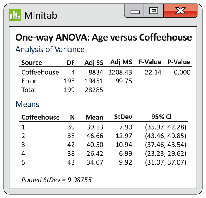
Figure 12.19 Minitab output for the coffeehouse study, Exercise 12.44.
-
In addition to the conditions of SRSs from each group and constant variance, which you already checked, the data must be approximately Normal. Do you think it is reasonable to assume that the data here are Normal? Include any plots or numeric summaries you use to answer this.
-
Write the null and alternative hypotheses associated with the F test in Figure 12.19.
-
Report the F statistic, its degrees of freedom, and the P-value. What are your conclusions?
-
-
12.45 Age differences across coffeehouses (continued). Recall the previous exercise. Using the estimates of the group means and
-
12.46 Time levels of scale. Recall Exercise 7.42 (page 429). This experiment actually involved three groups. The last group was told the construction project would last 12 months. Here is a summary of the interval lengths (in days) between the earliest and latest completion dates.

Group n s 52 weeks 30 84.1 55.8 12 months 30 104.6 70.1 1 year 30 139.6 73.1 -
Is this an observational study or an experiment? Explain your answer.
-
Use graphical methods to describe the three populations.
-
Examine the conditions necessary for ANOVA. Summarize your findings.
-
-
12.47 Time levels of scale (continued). Refer to the previous exercise.
Run the ANOVA and report the results.
-
Use a multiple-comparisons method to compare the three groups. State your conclusions.
-
The researchers hypothesized that the more fine-grained the time unit presented to a participant, the smaller the reported interval would be. To test this, they performed a simple linear regression using the group labels 1, 2, and 3 as the predictor variable. They found the slope
-
12.48 Facebook recruitment of young adult smokers. Studies about tobacco use have had difficulties recruiting young adults. Because Facebook is visited daily by a very large percent of young adults, researchers decided to investigate the effectiveness of using Facebook to recruit young adults for a smoking cessation trial. Thirty-six ads were run over a seven-week period, with each ad classified based on its image type. The effectiveness of each ad was assessed using the ad cost per unique click (CUC).

-
Figure 12.20 contains the JMP output for the analysis of the CUCs by image type. State your conclusions based on this output.
-
The researchers concluded that there were significant differences between the means for Cigarette and Logo and between the means for Cigarette and Social. Perform these comparisons using the least-significant differences (LSD) method. Do these comparisons have P-values below
-
Given your results in part (a), should the researchers report the results in part (b)? Explain your answer.
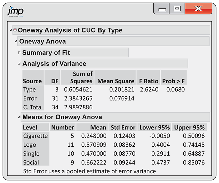
Figure 12.20 JMP one-way ANOVA output, Exercise 12.48.
-
-
12.49 Winery websites. As part of a study of British Columbia wineries, each of the 193 wineries was classified into one of three categories, based on its website features. The Presence stage just had information about the winery. The Portals stage included order placement and online feedback. The Transactions Integration stage included direct payment or payment through a third party online. The researchers then compared the number of market integration features of each winery (for example, in-house touring, a wine shop, a restaurant, in-house wine tasting, gift shop). Here are the results:15
Stage n s Presence 55 3.15 2.264 Portals 77 4.75 2.097 Transactions 61 4.62 2.346 -
Plot the means versus the stage of website. Does there appear to be a difference in the average number of market integration features?
-
Is this an observational study or an experiment? Explain your answer.
-
Is it reasonable to assume that the variances are equal? Justify your reasoning.
-
The data are counts (integer values). Also, based on the means and standard deviations, the distributions are skewed (can’t have a negative count). Do you think this lack of Normality poses a problem for ANOVA? Explain your answer.
-
The F statistic for these data is 9.594. Give the degrees of freedom and P-value. What do you conclude?
-
-
12.50 Which means differ significantly? Here is a table of means for a one-way ANOVA with four groups ordered from smallest to largest:
Group s n 1 128.2 7.7 20 4 135.0 8.6 20 2 142.1 8.7 20 3 148.6 10.8 20 Let’s compare the results using the two multiple-comparisons methods described in this chapter. Based on the table, the standard error for a comparison of two means is 2.853. Also, according to the LSD and Bonferroni multiple-comparisons methods with
-
Using the LSD method, mark the means of each pair of groups that do not differ significantly with the same letter. Summarize the results.
-
Using the Bonferroni method, mark the means of each pair of groups that do not differ significantly with the same letter. Summarize the results.
-
Do the results vary based on method? If so, which procedure results in more significantly different pairs of means? Explain why this is the case.
-
-
12.51 Financial incentives for weight loss. The use of financial incentives has shown promise in promoting weight loss and healthy behaviors. In one study, 104 employees of the Children’s Hospital of Philadelphia, with BMIs of 30 to 40 kilograms per square meter

-
Make a table giving the sample size, mean, and standard deviation for each program.
-
Is it reasonable to pool the variances? Explain your answer.
-
Generate a histogram for each of the programs. Can we feel confident that the sample means are approximately Normal? Defend your answer.
-
-
12.52 Financial incentives for weight loss (continued). Refer to the previous exercise.
-
Analyze the change in weight using analysis of variance. Report the test statistic, degrees of freedom, P-value, and your conclusions.
-
Even though you assessed the model assumptions in the previous exercise, let’s check the assumptions again by examining the residuals. Summarize your findings.
Compare the programs using the LSD method.
-
Using the results from parts (a), (b), and (c), write a short summary of your conclusions.
-
-
12.53 Changing the response variable. Refer to the previous two exercises, where we compared three weight-loss programs using change in weight measured in pounds. Suppose that you decide to instead make the comparison using change in weight measured in kilograms.
-
Convert the weight loss from pounds to kilograms by dividing each response by 2.2.
-
Analyze these new weight changes by using analysis of variance. Compare the test statistic, degrees of freedom, and P-value you obtain here with those reported in part (a) of the previous exercise. Summarize what you find.
-
-
 12.54 Do labels matter? A study was performed to
examine the self-identification of college students of Asian
descent with various identity categories and assess whether there
are attitudinal differences across these categories.
Undergraduates at a large midwestern university who had identified
themselves as being of Asian descent on their admission
application were asked to participate in the study.17
A total of 620 undergraduates filled out the survey. One question
classified the participants into groups by asking them to indicate
the option with which they primarily identify: (a) Asian American,
(b) specific ethnicity (for example, Chinese), (c) ethnicity
American (for example, Chinese American), and (d) other. The
responses to the remaining survey questions were then compared
across these four groups. One item was “The campus is supportive
of Asian American students.” Responses were on a four-point scale
12.54 Do labels matter? A study was performed to
examine the self-identification of college students of Asian
descent with various identity categories and assess whether there
are attitudinal differences across these categories.
Undergraduates at a large midwestern university who had identified
themselves as being of Asian descent on their admission
application were asked to participate in the study.17
A total of 620 undergraduates filled out the survey. One question
classified the participants into groups by asking them to indicate
the option with which they primarily identify: (a) Asian American,
(b) specific ethnicity (for example, Chinese), (c) ethnicity
American (for example, Chinese American), and (d) other. The
responses to the remaining survey questions were then compared
across these four groups. One item was “The campus is supportive
of Asian American students.” Responses were on a four-point scale
Label n Asian American 130 2.93 Specific ethnicity 248 3.00 Ethnicity American 174 3.01 Other 68 3.39 -
What are the numerator and denominator degrees of freedom for the F test?
-
Using the formula on page 617 and the preceding results, calculate SSG.
-
Given
-
Compute the P-value and state your conclusions.
-
Without doing any additional analysis, describe the pattern in the means that is likely responsible for your conclusions in part (d).
-
-
12.55 Do we experience emotions differently? Do people from different cultures experience emotions differently? One study designed to examine this question collected data from 410 college students from five different cultures.18 The participants were asked to record, on a 1 (never) to 7 (always) scale, how much of the time they typically felt eight specific emotions. These were averaged to produce the global emotion score for each participant. Here is a summary of this measure:
Culture n Mean (s) European American 46 4.39 (1.03) Asian American 33 4.35 (1.18) Japanese 91 4.72 (1.13) Indian 160 4.34 (1.26) Hispanic American 80 5.04 (1.16) Note that the convention of giving the standard deviations in parentheses after the means saves a great deal of space in a table such as this.
-
From the information given, do you think that we need to be concerned that a possible lack of Normality in the data will invalidate the conclusions that we might draw using ANOVA to analyze the data? Give reasons for your answer.
-
Is it reasonable to use a pooled standard deviation for these data? Why or why not?
-
The ANOVA F statistic was reported as 5.69. Give the degrees of freedom and either an approximate (from a table) or an exact (from software) P-value. Sketch a picture of the F distribution that illustrates the P-value. What do you conclude?
-
Without doing any additional formal analysis, describe the pattern in the means that appears to be responsible for your conclusion in part (c). Are there pairs of means that are quite similar?
-
-
12.56 The emotions study (continued). Refer to
the previous exercise. The experimenters also measured emotions in
some different ways. For a period of a week, each participant
carried a device that sounded an alarm at random times during a
three-hour interval five times a day. When the alarm sounded,
participants recorded several mood ratings indicating their
emotions for the time immediately preceding the alarm. These
responses were combined to form two variables: frequency, the
number of emotions recorded, expressed as a percent; and
intensity, an average of the intensity
scores measured on a scale of 0 to 6. At the end of the one-week
experimental period, the subjects were asked to recall the percent
of time that they experienced different emotions. This variable
was called “recall.” Here is a summary of the results:
Culture n Frequency mean (s) Intensity mean (s) Recall mean (s) European American 46 82.87 (18.26) 2.79 (0.72) 49.12 (22.33) Asian American 33 72.68 (25.15) 2.37 (0.60) 39.77 (23.24) Japanese 91 73.36 (22.78) 2.53 (0.64) 43.98 (22.02) Indian 160 82.71 (17.97) 2.87 (0.74) 49.86 (21.60) Hispanic American 80 92.25 (8.85) 3.21 (0.64) 59.99 (24.64) F statistic 11.89 13.10 7.06 -
For each response variable, state whether or not it is reasonable to use a pooled standard deviation to analyze these data. Give reasons for your answer.
-
Give the degrees of freedom for the F statistics and find the associated P-values. Summarize what you can conclude from these ANOVA analyses.
-
Summarize the means, paying particular attention to similarities and differences across cultures and across variables. Include the means from the previous exercise in your summary.
-
The European American and Asian American subjects were from the University of Illinois, the Japanese subjects were from two universities in Tokyo, the Indian subjects were from eight universities in or near Kolkata, and the Hispanic American subjects were from California State University at Fresno. Participants were paid $25 or an equivalent monetary incentive for the Japanese and Indian subjects. Ads were posted on or near the campuses to recruit volunteers for the study. Discuss how these facts influence your conclusions and the extent to which you would generalize the results.
-
The percents of female students in the samples were as follows: European American, 83%; Asian American, 67%; Japanese, 63%; Indian, 64%; and Hispanic American, 79%. Use a chi-square test to compare these proportions (see Section 9.2, page 506) and discuss how this information influences your interpretation of the results that you have found in this exercise.
-
-
12.57 Shopping and bargaining in Mexico. Price haggling and other bargaining behaviors among consumers have been observed for a long time. However, research addressing these behaviors, especially in a real-life setting, remains relatively sparse. A group of researchers performed a small study to determine whether gender or nationality of the bargainer has an effect on the final price obtained.19 The study took place in Mexico because of the prevalence of price haggling in informal markets. Salespersons working at various informal shops were approached by one of three bargainers looking for a specific product. After an initial price was stated by the vendor, bargaining took place. The response was the difference between the initial price and the final price of the product (in $US). The bargainers were a Spanish-speaking Hispanic male, a Spanish-speaking Hispanic female, and an Anglo non-Spanish-speaking male. The following table summarizes the results:
Bargainer n Average reduction Hispanic male 40 1.055 Anglo male 40 1.050 Hispanic female 40 2.310 -
To compare the mean reductions in price, what are the degrees of freedom for the ANOVA F statistic?
-
The reported test statistic is
-
To what extent do you think the results of this study can be generalized? Give reasons for your answer.
-
-
12.58 Restaurant ambiance and consumer behavior. Numerous studies have investigated the effects of restaurant ambiance on consumer behavior. One study investigated the effects of musical genre on consumer spending.20 At a single high-end restaurant in England over a three-week period, there were a total of 141 participants; 49 of them were subjected to background pop music (for example, Britney Spears, Culture Club, and Ricky Martin) while dining, 44 to background classical music (for example, Vivaldi, Handel, and Strauss), and 48 to no background music. For each participant, the total food bill, adjusted for time spent dining, was recorded. The following table summarizes the means and standard deviations (in British pounds):
Background music Mean bill n s Classical 24.130 44 2.243 Pop 21.912 49 2.627 None 21.697 48 3.332 Total 22.531 141 2.969 -
Plot the means versus the type of background music. Does there appear to be a difference in spending?
-
Is it reasonable to assume that the variances are equal? Explain.
-
The F statistic is 10.62. Give the degrees of freedom and either an approximate (from a table) or an exact (from software) P-value. What do you conclude?
-
Refer to part (a). Without doing any formal analysis, describe the pattern in the means that is likely responsible for your conclusion in part (c).
-
To what extent do you think the results of this study can be generalized to other settings? Give reasons for your answer.
-
-
12.59 Do isoflavones increase bone mineral density? Kudzu is a plant that was imported to the United States from Japan and now covers over 7 million acres in the South. The plant contains chemicals called isoflavones that have been shown to have beneficial effects on bones. One study used three groups of rats to compare a control group with rats that were fed either a low dose or a high dose of isoflavones from kudzu.21 One of the outcomes examined was the bone mineral density in the femur (in grams per square centimeter). Here are the data:

Treatment Bone mineral density Control 0.228 0.207 0.234 0.220 0.217 0.228 0.209 0.221 0.204 0.220 0.203 0.219 0.218 0.245 0.210 Low dose 0.211 0.220 0.211 0.233 0.219 0.233 0.226 0.228 0.216 0.225 0.200 0.208 0.198 0.208 0.203 High dose 0.250 0.237 0.217 0.206 0.247 0.228 0.245 0.232 0.267 0.261 0.221 0.219 0.232 0.209 0.255 -
Use graphical and numerical methods to describe the data.
-
Examine the assumptions necessary for ANOVA. Summarize your findings.
Run the ANOVA and report the results.
-
Use a multiple-comparisons method to compare the three groups.
-
Write a short report explaining the effect of kudzu isoflavones on the femur of the rat.
-
-
12.60 Do poets die young? According to William Butler Yeats, “She is the Gaelic muse, for she gives inspiration to those she persecutes. The Gaelic poets die young, for she is restless, and will not let them remain long on earth.” One study designed to investigate this issue examined the age at death for writers from different cultures and genders.22 Three categories of writers examined were novelists, poets, and nonfiction writers. Most of the writers were from the United States, but Canadian and Mexican writers were also included.

-
Use graphical and numerical methods to describe the data.
-
Examine the assumptions necessary for ANOVA. Summarize your findings.
Run the ANOVA and report the results.
-
Use a contrast to compare the poets with the two other types of writers. Do you think that the quotation from Yeats justifies the use of a one-sided alternative for examining this contrast? Explain your answer.
-
Use another contrast to compare the novelists with the nonfiction writers. Explain your choice for an alternative hypothesis for this contrast.
-
Use a multiple-comparisons method to compare the three means. How do the conclusions from this approach compare with those using the contrasts?
-
-
12.61 Exercise and healthy bones. Many studies have suggested that there is a link between exercise and healthy bones. Exercise stresses the bones, and this causes them to get stronger. One study examined the effect of jumping on the bone density of growing rats.23 There were three treatments: a control with no jumping, a low-jump condition (the jump height was 30 centimeters), and a high-jump condition (60 centimeters). After eight weeks of 10 jumps per day, five days per week, the bone density of the rats (expressed in milligrams per cubic centimeter) was measured. Here are the data:

Group Bone density Control 611 621 614 593 593 653 600 554 603 569 Low jump 635 605 638 594 599 632 631 588 607 596 High jump 650 622 626 626 631 622 643 674 643 650 -
Make a table giving the sample size, mean, and standard deviation for each group of rats. Is it reasonable to pool the variances?
-
Run the analysis of variance. Report the F statistic with its degrees of freedom and P-value. What do you conclude?
-
-
12.62 Exercise and healthy bones (continued). Refer to the previous exercise.
-
Examine the residuals. Is the Normality assumption reasonable for these data?
-
Use the Bonferroni method to determine which pairs of means differ significantly. Summarize your results in a short report. Be sure to include a graph.
-
-
12.63 Contrasts of interest. Refer to Exercise 12.57 (page 645). Given the group means and F statistic, we can determine that
Test if there is a difference between the sexes.
-
Test if there is a difference between nationalities.
-
Explain why this study would have benefited from also including an Anglo female bargainer.
-
12.64 Public transit use and physical activity. In one study on physical activity, participants used accelerometers and a seven-day travel log to monitor their physical activity.24 Researchers used the data from each participant to quantify the amount of daily physical activity and to classify each participant as a nontransit user or a low-, mid-, or high-frequency transit user. Here is a summary of physical activity (in minutes per day) broken down into walking and nonwalking activities. One-way ANOVA was used to compare the groups across each activity.
Physical activity Nontransit Low frequency Mid frequency High frequency Overall P-value Walking Nonwalking 16.0 13.5 11.9 15.2 0.24 -
Would this be considered an observational study or an experiment? Explain your answer.
-
What are the numerator and denominator degrees of freedom for the F tests?
-
State the null and alternative hypotheses associated with each of the overall P-values.
-
The superscript letters in each row summarize the multiple-comparisons results. Write a short paragraph explaining what these results tell you with regard to walking and nonwalking physical activity.
-
-
12.65 A comparison of different types of scaffold material. One way to repair serious wounds is to insert some material as a scaffold for the body’s repair cells to use as a template for new tissue. Scaffolds made from extracellular material (ECM) are particularly promising for this purpose. Because they are made from biological material, they serve as an effective scaffold and are then resorbed. Unlike biological material that includes cells, however, they do not trigger tissue rejection reactions in the body. One study compared six types of scaffold material.25 Three of these were ECMs, and the other three were made of inert materials (MAT). There were three mice used per scaffold type. The response measure was the percent of glucose phosphated isomerase (Gpi) cells in the region of the wound. A large value is good, indicating that there are many bone marrow cells sent by the body to repair the tissue.

Material Gpi (%) ECM1 55 70 70 ECM2 60 65 65 ECM3 75 70 75 MAT1 20 25 25 MAT2 5 10 5 MAT3 10 15 10 -
Make a table giving the sample size, mean, and standard deviation for each of the six types of material. Is it reasonable to pool the variances? Note that the sample sizes are small and the data are rounded.
-
Run the analysis of variance. Report the F statistic with its degrees of freedom and P-value. What do you conclude?
-
-
12.66 A comparison of different types of scaffold material (continued). Refer to the previous exercise.
-
Examine the residuals. Is the Normality assumption reasonable for these data?
-
Use the Bonferroni or another multiple-comparisons method to determine which pairs of means differ significantly. Summarize your results in a short report. Be sure to include a graph.
-
Use a contrast to compare the three ECM materials with the three other materials. Summarize your conclusions. How do these results compare with those that you obtained from the multiple-comparisons method in part (b)?
-
-
12.67 The two-sample t test and one-way ANOVA. Refer to the diet and mood study in Exercise 7.48 (page 430). Find the two-sample pooled t statistic for comparing the two energy-restricted diets. Then formulate the problem as an ANOVA and report the results of this analysis. Verify that
-
12.68 A dandruff study. Analysis of variance methods are often used in clinical trials where the goal is to assess the effectiveness of one or more treatments for a particular medical condition. One such study compared three treatments for dandruff and a placebo. The treatments were 1% pyrithione zinc shampoo (PyrI), the same shampoo but with instructions to shampoo two times (PyrII), 2% ketoconazole shampoo (Keto), and a placebo shampoo (Placebo). After six weeks of treatment, eight sections of the scalp were examined and given a score that measured the amount of scalp flaking on a 0 to 10 scale. The response variable was the sum of these eight scores. An analysis of the baseline flaking measure indicated that randomization of patients to treatments was successful in that no differences were found between the groups. At baseline, there were 112 subjects in each of the three treatment groups and 28 subjects in the Placebo group. During the clinical trial, three dropped out from the PyrII group and six from the Keto group. No patients dropped out of the other two groups.

-
Find the mean, standard deviation, and standard error for the subjects in each group. Summarize these, along with the sample sizes, in a table and make a graph of the means.
-
Run the analysis of variance on these data. Write a short summary of the results and your conclusion. Be sure to include the hypotheses tested, the test statistic with degrees of freedom, and the P-value.
-
-
12.69 The dandruff study (continued). Refer to the previous exercise.
-
Plot the residuals versus case number (the first variable in the data set). Describe the plot. Is there any pattern that would cause you to question the assumption that the data are independent?
-
Examine the standard deviations for the four treatment groups. Is there a problem with the assumption of equal standard deviations for ANOVA in this data set? Explain your answer.
-
Create Normal quantile plots for each treatment group. What do you conclude from these plots?
-
Obtain the residuals from the analysis of variance and create a Normal quantile plot of these. What do you conclude?
-
-
12.70 Comparing each pair of dandruff treatments. Refer to Exercise 12.68. Use the Bonferroni or another multiple-comparisons method that your software provides to compare the individual group means in the dandruff study. Write a short summary of your conclusions.
-
12.71 Testing several contrasts from the dandruff study. Refer to Exercise 12.68. There are several natural contrasts in this experiment that describe comparisons of interest to the experimenters. They are (1) Placebo versus the average of the other three treatments, (2) Keto versus the average of the two Pyr treatments, and (3) PyrI versus PyrII.
-
Express each of these three contrasts in terms of the means
-
Give estimates with standard errors for each of the contrasts.
-
Perform the significance tests for the contrasts. Summarize the results of your tests and your conclusions.
-
-
12.72 Changing the response variable. Refer to Exercise 12.65 (page 647), where we compared six types of scaffold material to repair wounds. The data are given as percents ranging from 5 to 75.
-
Convert these percents into their decimal form by dividing by 100. Calculate the transformed means, standard deviations, and standard errors and summarize them, along with the sample sizes, in a table.
-
Explain how you could have calculated the table entries directly from the table you gave in part (a) of Exercise 12.65.
-
Analyze the decimal forms of the percents using analysis of variance. Compare the test statistic, degrees of freedom, P-value, and conclusion you obtain here with the corresponding values that you found in Exercise 12.65.
-
-
12.73 More on changing the response variable. Refer to the previous Exercise and Exercise 12.65 (page 647). A calibration error was found with the device that measured Gpi, which resulted in a shifted response. Add 5% to each response and redo the calculations. Summarize the effects of transforming the data by adding a constant to all responses.
-
12.74 Linear transformation of the response variable.
Refer to the previous two Exercises. Can you suggest a general
conclusion regarding what happens to the test statistic, degrees
of freedom, P-value, and conclusion when you perform
analysis of variance on data that have been transformed by
multiplying the raw data by a constant and then adding another
constant? (That is, if y is the original data, we analyze
y*, where
-
12.75 Planning another emotions study. Scores on an emotional scale were compared for five different cultures in Exercise 12.55 (page 644). Suppose that you are planning a new study using the same outcome variable. Your study will use European American, Asian American, and Hispanic American students from a large university.
-
Explain how you would select the students to participate in your study.
-
Use the data from Exercise 12.55 to perform power calculations to determine sample sizes for your study.
-
Write a report that could be understood by someone with limited background in statistics and that describes your proposed study and why you think it is likely that you will obtain interesting results.
-
-
12.76 Planning another isoflavone study.
Exercise12.59 (page 645) gave data for a bone health study that examined the effect of
isoflavones on rat bone mineral density. In this study, there were
three groups. Controls received a placebo, and the other two
groups received either a low dose or a high dose of isoflavones
from kudzu. You are planning a similar study of a new kind of
isoflavone. Use the results of the study described in
Exercise 12.59 to plan
your study. Write a proposal explaining why your study should be
funded.
-
12.77 Planning another restaurant ambiance study.
Exercise 12.58 (page 645) gave data for a study that examined the effect of background
music on total food spending at a high-end restaurant. You are
planning a similar study but intend to look at total food spending
at a more casual restaurant. Use the results of the study
described in
Exercise 12.58 to plan
your study.
-
12.78 The noncentral F distribution. The noncentral F distribution is defined by three parameters: the numerator and denominator degrees of freedom and a noncentrality parameter
Large
-
What are the numerator and denominator degrees of freedom for these two Exercises, given
-
Using the information in the Exercises and
-
Using these values of
-
PUTTING IT ALL TOGETHER
-
12.79 The effect of music on risky financial decisions. Decisions regarding investments involve some degree of risk. The degree of risk someone is willing to accept is related to the individual’s mood and arousal. Because music has been shown to influence both mood and arousal, researchers were interested in the effects of high- and low-arousal music on financial decisions.27 In one experiment, participants were randomly assigned to either low-tempo music, high-tempo music, or a no music control group. After listening to the music for a couple of minutes, the participants were asked to allocate 100 coins between a risky asset and a risk-free asset. The number of coins assigned to the risky asset (Coin) is the response variable of interest. Using the tools of this chapter, analyze the data and present a short summary of your findings.

-
12.80 Massage therapy for osteoarthritis of the knee. Various studies have shown the benefits of massage to manage pain. In one study, 125 adults suffering from osteoarthritis of the knees were randomly assigned to one of five eight-week regimens.28 The primary outcome was the decrease in the Western Ontario and McMaster Universities Arthritis Index (WOMAC-Global). This index is used extensively to assess pain and functioning in those suffering from arthritis. Positive values indicate improvement. The following table summarizes the results of those completing the study:
Regimen n s 30 min massage 22 17.4 17.9 30 min massage 24 18.4 20.7 60 min massage 24 24.0 18.4 60 min massage 25 24.0 19.8 Usual care, no massage 24 6.3 14.6 -
What proportion of adults dropped out of the study before completion?
-
Is it reasonable to use the assumption of equal standard deviations when we analyze these data? Give a reason for your answer.
Find the pooled standard deviation.
-
The
-
There are 10 pairs of means to compare. For the Bonferroni multiple-comparisons method, the critical t-value is 2.863. Which pairs of means are found to be significantly different? Write a short summary of your analysis.
-
-
12.81 Contrasts for the massage study. Refer to the previous Exercise. There are several comparisons of interest in this study. They are (1) usual care versus the average of the massage groups; (2) the average of the two 30-minute massage groups versus the average of the two 60-minute massage groups; and (3) the difference between a 30-minute massage once a week and twice a week versus the difference between a 60-minute massage once a week and twice a week.
-
Express each contrast in terms of the means
-
Give estimates with standard errors for each of the contrasts.
-
Perform the significance tests for the contrasts. Summarize the results of your tests and your conclusions.
-