7.2 Comparing Two Means
A psychologist wants to compare Wisconsin and Indiana college students’ impressions of personality based on selected Facebook pages. A nutritionist is interested in the effect of increased calcium on blood pressure. A bank wants to know which of two incentive plans will most increase the use of its debit card. Two-sample problems such as these are among the most common situations encountered in statistical practice.
A two-sample problem can arise from a randomized comparative experiment that randomly divides the subjects into two groups and exposes each group to a different treatment. A two-sample problem can also arise when comparing random samples separately selected from two populations. Unlike in the matched pairs designs studied earlier, there is no matching of the units in the two samples. In fact, the two samples may be of different sizes. As a result of these differences, inference procedures for two-sample data differ from those for matched pairs.
We can present two-sample data graphically by using a back-to-back stemplot for small samples (page 13) or with side-by-side boxplots for larger samples (page 34). Now we will apply the ideas of formal inference in this setting. When both population distributions are symmetric, and especially when they are at least approximately Normal, a comparison of the mean responses in the two populations is most often the goal of inference.
We have two independent samples, from two distinct populations (such as
subjects given the latest Apple iPhone and those given the latest
Samsung Galaxy smartphone). The same response variable—say, battery
life—is measured for both samples. We will call the variable
| Population | Variable | Mean | Standard deviation |
|---|---|---|---|
| 1 |
|
|
|
| 2 |
|
|
|
We want to compare the two population means, either by giving a
confidence interval for
Inference is based on two independent SRSs, one from each population. Here is the notation that describes the samples:
| Population | Sample size | Sample Mean | Sample standard deviation |
|---|---|---|---|
| 1 |
|
|
|
| 2 |
|
|
|
Throughout this section, the subscripts 1 and 2 show the population to which a parameter or a sample statistic refers.
The two-sample z statistic
The natural estimator of the difference
-
The mean of the difference
-
The variance of the difference
-
Because the samples are independent, their sample means
-
If the two population distributions are both Normal, then the distribution of
We now know the sampling distribution of
Here’s an example of a Normal distribution probability calculation using this sampling distribution.
Example 7.13 Heights of 10-year-old girls and boys.

A fourth-grade class has 12 girls and 8 boys. The children’s heights are recorded on their 10th birthdays. What is the chance that the girls are taller than the boys? Of course, it is very unlikely that all the girls are taller than all the boys. We translate the question into the following: What is the probability that the mean height of the girls in this class is greater than the mean height of the boys in this class?
Based on information from the National Health and Nutrition Examination Survey, we assume that the heights (in inches) of 10-year-old girls are N(56.9, 2.8) and the heights of 10-year-old boys are N(56.0, 3.5).23 The heights of the students in our class are assumed to be random samples from these populations. The two distributions are shown in Figure 7.13(a).
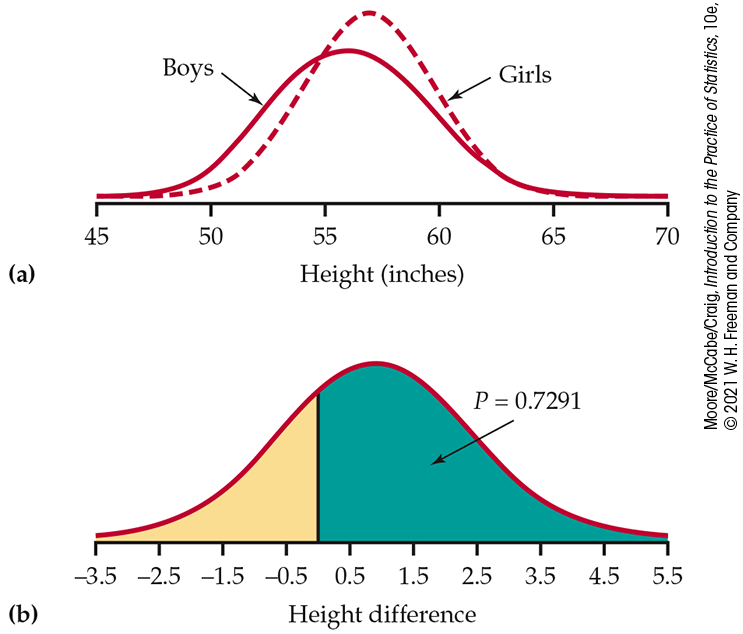
Figure 7.13 Distributions, Example 7.13. (a) Distributions of heights of 10-year-old boys and girls. (b) Distribution of the difference between mean heights of 12 girls and 8 boys.
The difference
and variance
The standard deviation of the difference in sample means is,
therefore,
If the heights vary Normally, the difference in sample means is also
Normally distributed. The distribution of the difference in heights
is shown in
Figure 7.13(b). We standardize
Even though the population mean height of 10-year-old girls is greater than the population mean height of 10-year-old boys, the probability that the sample mean of the girls is greater than the sample mean of the boys in our class is only 73%. Large samples are needed to see the effects of small differences.
As Example 7.13 reminds us, any Normal random variable has the N(0, 1) distribution when standardized. We have arrived at a new z statistic.
In the unlikely event that both population standard deviations are
known, the two-sample z statistic is the basis for inference
about
The two-sample t procedures
![]()
Suppose now that the population standard deviations
Unfortunately, this statistic does not have a
t distribution. A t distribution replaces the
N(0, 1) distribution only when a single standard
deviation is replaced by its estimate. In this case, we replace
two standard deviations
Nonetheless, we can approximate the distribution of the two-sample
t statistic by using the t(k) distribution with
an approximation for the degrees of freedom k, also known as a
df
approximation. We use these approximations to find approximate values of
Most statistical software uses the Satterthwaite approximation to approximate the t(k) distribution unless the user requests another method. Use of this approximation without software is a bit complicated.24 In general, the resulting k will not be an integer.
If you cannot access software, we recommend using degrees of freedom
k equal to the smaller of
The two-sample t confidence interval
We now apply the basic ideas about t procedures to the problem of comparing two means when the standard deviations are unknown. Just as we did in the one-sample case, we start with confidence intervals.
Example 7.14 Directed reading activities assessment.
![]()
An educator believes that new directed reading activities in the classroom will help elementary school pupils improve some aspects of their reading ability. She arranges for a third-grade class of 21 students to take part in these activities for an eight-week period. A control classroom of 23 third-graders follows the same curriculum without the activities. At the end of the eight weeks, all students are given a Degree of Reading Power (DRP) test, which measures the aspects of reading ability that the treatment is designed to improve. The data appear in TABLE 7.4.26
| Treatment group | Control group | ||||||
|---|---|---|---|---|---|---|---|
| 24 | 61 | 59 | 46 | 42 | 33 | 46 | 37 |
| 43 | 44 | 52 | 43 | 43 | 41 | 10 | 42 |
| 58 | 67 | 62 | 57 | 55 | 19 | 17 | 55 |
| 71 | 49 | 54 | 26 | 54 | 60 | 28 | |
| 43 | 53 | 57 | 62 | 20 | 53 | 48 | |
| 49 | 56 | 33 | 37 | 85 | 42 | ||
Prior to inference, we need to check whether the t procedures can be used for these data. The following back-to-back stemplot suggests that there is a mild outlier in the control group but no deviation from Normality serious enough to forbid use of t procedures. Separate Normal quantile plots for both groups (Figure 7.14) confirm that both distributions are approximately Normal.
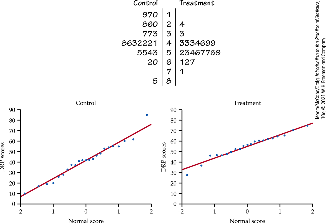
Figure 7.14 Normal quantile plots of the DRP scores, Example 7.14.
The design of the study in Example 7.14 is not ideal. Random assignment of students was not possible in a school environment, so existing third-grade classes were used. The effect of the reading programs is, therefore, confounded with any other differences between the two classes. That said, the classes were chosen to be as similar as possible—for example, in terms of the social and economic status of the students. Extensive pretesting also showed that the two classes were, on the average, quite similar in reading ability at the beginning of the experiment. To avoid the effect of two different teachers, the researcher herself taught reading in both classes during the eight-week period of the experiment. Therefore, we can be somewhat confident that the two-sample test is detecting the effect of the treatment and not some other difference between the classes. This example is typical of many situations in which an experiment is carried out but randomization is not possible.
Example 7.15 Computing an approximate 95% confidence interval for the difference in means.
![]()
From our examination of the data in Example 7.14, the scores of treatment group appear to be somewhat higher than those of the control. The summary statistics are
| Group | n |
|
s |
|---|---|---|---|
| Treatment | 21 | 51.48 | 11.01 |
| Control | 23 | 41.52 | 17.15 |
To describe the size of the treatment effect, let’s construct a confidence interval for the difference between the treatment group and the control group means. The interval is
Using software, the degrees of freedom are 37.86 and
The conservative approach would use the smaller of
Table D
gives
|
|
|||
|
|
1.725 | 2.086 | 2.197 |
| C | 0.90 | 0.95 | 0.96 |
With this approximation, we have
The conservative approach gives a slightly wider interval than the more accurate approximation used by software. However, the difference is very small. We estimate the mean improvement to be about 10 points, with a margin of error of almost 9 points. Unfortunately, the data do not allow a very precise estimate of the size of the average improvement.
Check-in
-
7.15 Two-sample t confidence interval. Suppose a study similar to Example 7.14 were performed using two second-grade classes. Assume that the summary statistics are
-
7.16 Smaller sample sizes. Refer to the previous Check-in question. Suppose instead that the two classes are smaller but the summary statistics do not change:
The two-sample t significance test
The same ideas that we used for the two-sample t confidence interval also apply to the two-sample t significance test. We can use either software or the conservative approach with Table D to approximate the P-value.
Example 7.16 Is there an improvement?
![]()
For the DRP study described in Example 7.14 (page 414), we hope to show that the treatment (Group 1) performs better than the control (Group 2). For the two-sample t significance test, the same set of hypotheses can be presented as
The two-sample t statistic is
The P-value for the one-sided test is
|
|
||
| p | 0.02 | 0.01 |
|
|
2.197 | 2.528 |
Without software, we’d again use 20 degrees of freedom. Comparing 2.31 with the row entries in Table D, we see that P lies between 0.01 and 0.02.
The data strongly suggest that directed reading activity improves
the DRP score
Check-in
-
7.17 A two-sample t significance test. Refer to Check-in question 7.15. Perform a significance test at the 0.05 level to assess whether the average improvement is five points versus the alternative that it is greater than five points. Write a one-sentence conclusion.
-
7.18 Interpreting the confidence interval. Refer to the previous Check-in question. Can the confidence interval in Check-in question 7.15 (page 416) be used to determine whether the significance test of the previous Check-in question rejects or does not reject the null hypothesis? Explain your answer.
Most statistical software requires the raw data for analysis. A few, like Minitab, will also perform a t test on data in summarized form (such as the summary statistics table in Example 7.15). It is always preferable to work with the raw data because one can also examine the data through plots such as the back-to-back stemplot and Normal quantile plots in Example 7.14.
Example 7.17 Using software.
![]()
Figure 7.15 shows JMP and Minitab outputs for the comparison of DRP scores. Both outputs include the 95% confidence interval and the significance test that the means are equal. JMP reports the difference as the mean of treatment minus the mean of control, while Minitab reports the difference in the opposite order.
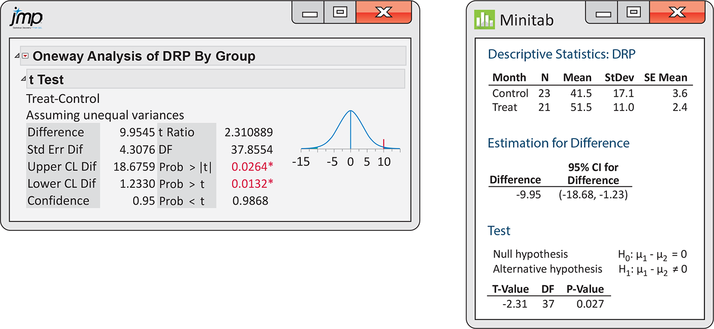
Figure 7.15 JMP and Minitab outputs, Example 7.17.
Recall that the confidence interval (treatment minus control) is
From the JMP output, we see that the degrees of freedom under the
first approximation are 37.86. Minitab also uses the first degrees
of freedom approximation but rounds the degrees of freedom down to
the nearest integer
The default Minitab output only considers the two-sided alternative.
Our test in
Example 7.16
is one-sided. If your software gives you the P-value for only
the two-sided alternative,
Robustness of the two-sample procedures
The two-sample t procedures are more robust than the one-sample
t methods. When the sizes of the two samples are equal and the
distributions of the two populations being compared have similar
shapes, probability values from the t
table are quite accurate for a broad range of distributions when the
sample sizes are as small as
-
If
-
If
-
Large samples
These guidelines are rather conservative, especially when the two samples are of equal size. In planning a two-sample study, choose equal sample sizes if you can. The two-sample t procedures are most robust against non-Normality in this case, and the conservative probability values are most accurate.
Here is an example with sample sizes that are almost equal and whose total sample size is more than 40. Even if the distributions are not Normal, we are confident that the sample means will be approximately Normal. The two-sample t procedures are very robust in this case.
Example 7.18 Low-calorie sweeteners and body weight.
![]()
Low-calorie sweeteners (LCSs) are commonly used as sugar substitutes because they provide sweetness with little or no energy. The unique chemical structure of each LCS, however, may evoke different sensory and behavioral responses that could affect body weight. To study this, a 12-week randomized trial was run to compare 4 LCSs and sugar.28 We will just focus on two of the LCSs (saccharin and sucralose) for this example.
Each day, participants were asked to also consume a sweetened beverage in addition to their normal diet. Here are the summary statistics of the weight change over the 12 weeks, in kilograms (kg):
| Group | n |
|
s |
|---|---|---|---|
| Saccharin | 25 | 1.17 | 2.56 |
| Sucralose | 24 |
|
2.84 |
Those who consumed sucralose lost slightly less than a kilogram, while those who consumed saccharin gained slightly more than a kilogram. Can we conclude that these two groups are not the same? Or is this difference what we could expect to see, given the variation among participants?
The researchers did not specify a direction for the difference. Thus, the hypotheses are
Figure 7.16
contains the Normal quantile plots for each group. There are no
obvious outliers, and the distributions are reasonably Normal.
However, given that the sum of the samples is large
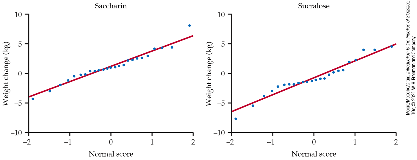
Figure 7.16 Normal quantile plots, Example 7.18.
The two-sample t statistic is
The conservative approach finds the P-value by comparing 2.60
to critical values for the t(23) distribution because the
smaller sample has 24 observations. Using
Table D
we find
|
|
||
| p | 0.01 | 0.005 |
|
|
2.500 | 2.807 |
The data give strong evidence that saccharin results in a larger
weight change than sucralose
In this and other examples, we can choose which population to label 1
and which to label 2. After inspecting the data, we chose saccharin
consumers as Population 1 because this choice makes the
t statistic a positive number. This avoids any possible
confusion from reporting a negative value for t.
![]() Choosing the population labels is not the same as choosing a
one-sided alternative after looking at the data.
Choosing hypotheses after seeing a result in the data is a violation
of sound statistical practice.
Choosing the population labels is not the same as choosing a
one-sided alternative after looking at the data.
Choosing hypotheses after seeing a result in the data is a violation
of sound statistical practice.
Inference for small samples
Small samples require special care. We do not have enough observations to examine the distribution shapes, and only extreme outliers stand out. The power of significance tests tends to be low, and the margins of error of confidence intervals tend to be large. Despite these difficulties, we can often draw important conclusions from studies with small sample sizes. If the size of an effect is very large, it should still be evident even if the n’s are small.
Example 7.19 A small study of LCSs and body weight.
![]()
In the setting of Example 7.18, let’s consider a much smaller study that collects weight change data from only five participants in each LCS group. Also, given the results of this past example, we choose the one-sided alternative. The data are
| Group | Weight change (kg) | ||||
|---|---|---|---|---|---|
| Saccharin | 0.5 | 3.0 | 4.2 | 2.3 | 3.3 |
| Sucralose | 0.1 | 1.2 |
|
|
|
First, examine the distributions with a back-to-back stemplot
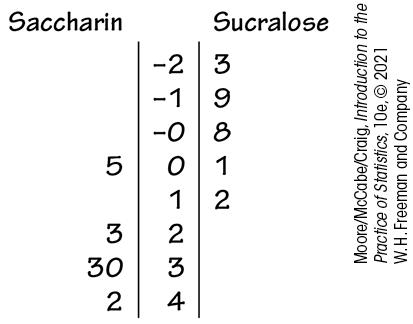
While there is variation among weight changes within each group, there is also a noticeable separation. The saccharin group contains four of the five largest weight gains, and the sucralose group contains four of the five smallest losses. A significance test can confirm whether this pattern can arise just by chance or if the saccharin group has a higher mean. We test
The average weight change is higher in the saccharin group
Figure 7.17 gives outputs for this analysis from four software packages. Although the formats differ, the basic information is the same. All report the sample sizes, the sample means and standard deviations (or variances), the t statistic, and its P-value. All agree that the P-value is small, though some outputs give more detail than others. Software often labels the groups in alphabetical order. Always check the means first and report the statistic (you may need to change the sign) in an appropriate way. Be sure to also mention the size of the effect you observed, such as “The mean weight change for the saccharin group was 3.40 kg higher than for the sucralose group.”
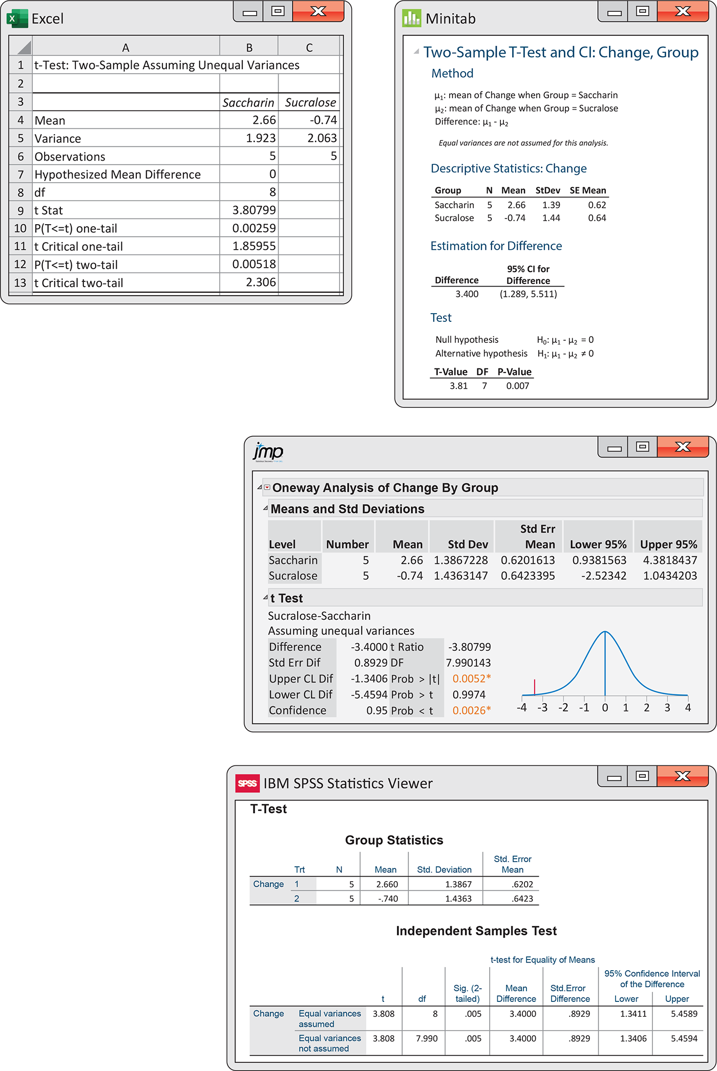
Figure 7.17 Excel, Minitab, JMP, and SPSS outputs, Example 7.19.
The SPSS output reports the results of two t procedures: the
general two-sample procedure that we have just studied and a special
procedure which assumes that the two population variances are equal.
The “equal-variances” procedures are most helpful in cases like this
when the sample sizes
The pooled two-sample t procedures
Suppose that the two Normal population distributions whose means we want to compare have the same standard deviation. How does this additional condition impact our t statistic? Let’s investigate! As we did with the general procedure, we’ll first develop the z statistic and from it the t statistic.
Let’s call the common—but unknown—standard deviation
The standardized difference of means is therefore
This is the special two-sample z statistic for the case in
which the populations have the same
To get to the t statistic, we replace the unknown
This is called the
pooled
estimator of
Because we replace a single standard deviation
Example 7.20 Calcium and blood pressure.
![]()

Does increasing the amount of calcium in our diet reduce blood pressure? Examination of a large sample of people revealed a relationship between calcium intake and blood pressure, but such observational studies do not establish causation. Animal experiments, however, showed that calcium supplements do reduce blood pressure in rats, justifying an experiment with human subjects. A randomized comparative experiment gave one group of 10 black men a calcium supplement for 12 weeks. The control group of 11 black men received a placebo that appeared identical. (In fact, a block design with black and white men as the blocks was used. We will look only at the results for the black men because an earlier survey suggested that calcium is more effective for blacks.) The experiment was double-blind. TABLE 7.5 gives the seated systolic (heart contracted) blood pressure for all subjects at the beginning and end of the 12-week period, in millimeters of mercury (mm Hg). Because the researchers were interested in decreasing blood pressure, Table 7.5 also shows the decrease for each subject. An increase appears as a negative entry.29
| Calcium group | Placebo group | ||||
|---|---|---|---|---|---|
| Begin | End | Decrease | Begin | End | Decrease |
| 107 | 100 | 7 | 123 | 124 |
|
| 110 | 114 |
|
109 | 97 | 12 |
| 123 | 105 | 18 | 112 | 113 |
|
| 129 | 112 | 17 | 102 | 105 |
|
| 112 | 115 |
|
98 | 95 | 3 |
| 111 | 116 |
|
114 | 119 |
|
| 107 | 106 | 1 | 119 | 114 | 5 |
| 112 | 102 | 10 | 114 | 112 | 2 |
| 136 | 125 | 11 | 110 | 121 |
|
| 102 | 104 |
|
117 | 118 |
|
| 130 | 133 |
|
|||
As usual, we first examine the data. To compare the effects of the two treatments, take the response variable to be the amount of the decrease in blood pressure. Inspection of the data reveals that there are no outliers. Side-by-side boxplots and Normal quantile plots (Figures 7.18 and 7.19) give a more detailed picture. The calcium group has a somewhat short left tail, but there are no severe departures from Normality that will prevent use of t procedures.
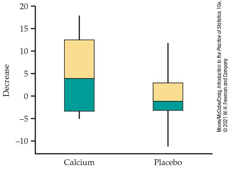
Figure 7.18 Side-by-side boxplots of the decrease in blood pressure from Table 7.5.
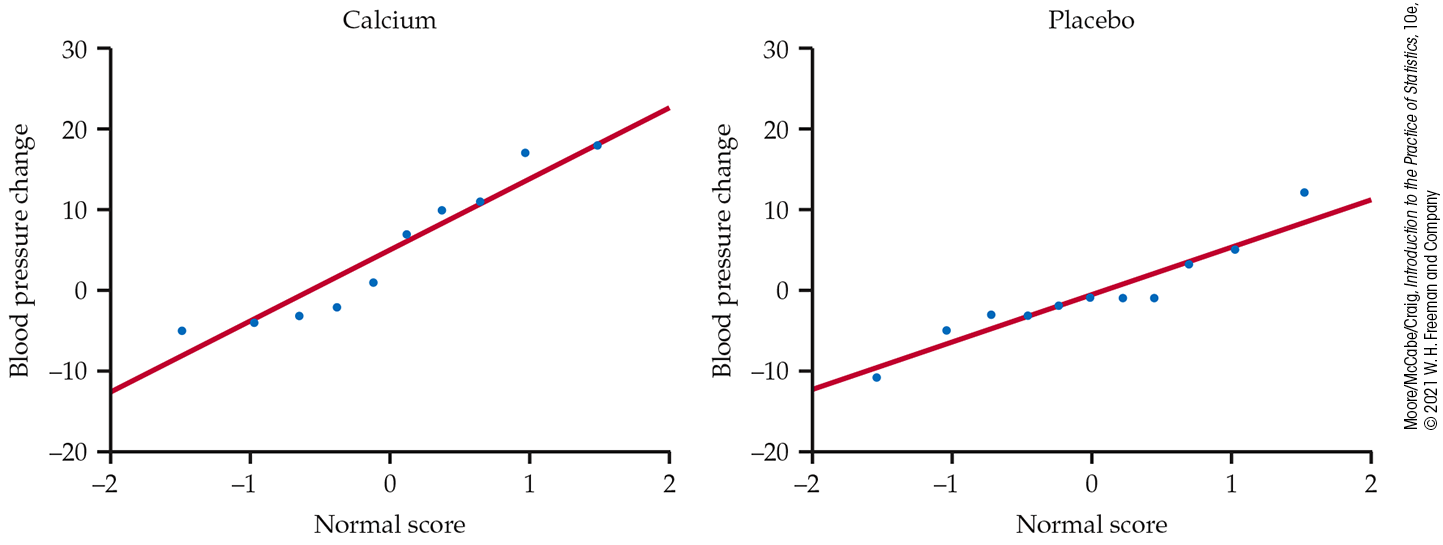
Figure 7.19 Normal quantile plots of the change in blood pressure from Table 7.5.
To examine the question of the researchers who collected these data, we perform a significance test.
Example 7.21 Does increased calcium reduce blood pressure?
![]()
Take Group 1 to be the calcium group and Group 2 to be the placebo group. The evidence that calcium lowers blood pressure more than a placebo is assessed by testing
Here are the summary statistics for the decrease in blood pressure:
| Group | Treatment | n |
|
s |
|---|---|---|---|---|
| 1 | Calcium | 10 | 5.000 | 8.743 |
| 2 | Placebo | 11 |
|
5.901 |
The calcium group shows a drop in blood pressure, and the placebo group has a small increase. The sample standard deviations do not rule out equal population standard deviations. A difference this large will often arise by chance in samples this small. We are willing to assume equal population standard deviations. The pooled sample variance is
so that
The pooled two-sample t statistic is
The P-value is
|
|
||
| p | 0.10 | 0.05 |
|
|
1.328 | 1.729 |
Sample size strongly influences the P-value of a test. An
effect that fails to be significant at a specified level
Of course, a P-value is almost never the last part of a statistical analysis. To make a judgment regarding the size of the effect of calcium on blood pressure, we need a confidence interval.
Example 7.22 How different are the calcium and placebo groups?
![]()
We estimate that the effect of calcium supplementation is the
difference between the sample means of the calcium and the placebo
groups,
We are 90% confident that the difference in means is in the interval
The pooled two-sample t procedures are anchored in
statistical theory and so have long been the standard version of the
two-sample t in textbooks.
![]() These procedures, however, require the condition that the two
unknown population standard deviations are equal.
This condition is hard to verify.
These procedures, however, require the condition that the two
unknown population standard deviations are equal.
This condition is hard to verify.
The pooled t procedures are, therefore, a bit risky. They are reasonably robust against both non-Normality and unequal standard deviations when the sample sizes are nearly the same. When the samples are quite different in size, the pooled t procedures become sensitive to unequal standard deviations and should be used with caution unless the samples are large. Unequal standard deviations are very common. In particular, it is not unusual for the spread of data to increase when the center of the data increases. We recommend regular use of the general t procedures, particularly when software automates the Satterthwaite approximation.
Check-in
-
7.19 Using software. Figure 7.17 (page 422) gives the outputs from four software packages for comparing the weight change of two groups consuming different low-calorie sweeteners. For the general two-sample t test, all software use the Satterthwaite approximation for degrees of freedom, but some round down or to the nearest integer. Summarize what each software does and provide its P-value.
-
7.20 Let’s consider the pooled t test. Example 7.18 (page 419) gives summary statistics for the weight change in two low-calorie sweetener groups. The two sample standard deviations are relatively close, so we may be willing to assume equal population standard deviations. Calculate the pooled t statistic and its degrees of freedom from the summary statistics. Use Table D to assess significance. How do your results compare with the unpooled analysis for these data?
Section 7.2 SUMMARY
-
Significance tests and confidence intervals for the difference between the means
-
When independent SRSs of sizes
has the N(0, 1) distribution.
-
The two-sample t statistic
does not have a t distribution. However, software can give accurate P-values using the Satterthwaite approximation.
-
Conservative inference procedures for comparing
-
An approximate level C confidence interval for
Here,
-
Significance tests for
The P-value is approximated using the t(k) distribution, where k is determined from the data by software or is the smaller of
-
The guidelines for practical use of two-sample t procedures are similar to those for one-sample t procedures. Equal sample sizes are recommended.
-
If we can consider that the two populations have equal variances, the pooled two-sample t procedures can be used. These are based on the pooled estimator of
and the
Section 7.2 EXERCISES
In these two-sample t problems, try to use the degrees of freedom
approximation provided by software. For exercises involving
summarized data, this approximation is provided for you. If you
instead use the conservative approximation, the smaller of
-
7.35 What’s wrong? For each of the following statements, explain what is wrong and why.
-
A researcher wants to test
-
A study recorded the IQ scores of 100 college freshmen. The scores of the 56 males in the study were compared with the scores of all 100 freshmen using the two-sample methods of this section.
-
A two-sample t statistic gave a P-value of 0.94. From this, we can reject the null hypothesis with 90% confidence.
-
A researcher is interested in testing the one-sided alternative
-
-
7.36 Basic concepts. For each of the following, answer the question and give a short explanation of your reasoning.
-
A 95% confidence interval for the difference between two means is reported as (0.8, 2.3). What can you conclude about the results of a significance test of the null hypothesis that the population means are equal versus the two-sided alternative?
-
Will larger samples generally give a larger or smaller margin of error for the difference between two sample means?
-
-
7.37 More basic concepts. For each of the following, answer the question and give a short explanation of your reasoning.
-
A significance test for comparing two means gave
-
Answer part (a) for the one-sided alternative that the difference between means is negative.
-
-
7.38 Physical demands of women’s rugby sevens matches. Rugby sevens is rapidly growing in popularity and became an Olympic sport in 2016. Matches are played on a full rugby field and consist of two seven-minute halves. Each team also consists of seven players. To better understand the demands of women’s rugby sevens, a group of researchers compared the physical qualities of elite players from the Canadian National team with a university squad. The following table summarizes some of these qualities:30
Quality Elite University s s Sprint speed (km/hr) 27.3 0.7 26.0 1.5 Peak heart rate (bpm) 192.0 6.0 193.0 6.0 Intermittent recovery test (m) 1160 191 781 129 Carry out the significance tests using
-
7.39 Noise levels in fitness classes. Fitness classes often have very loud music that could affect hearing. One study collected noise levels (decibels) in both high-intensity and low-intensity fitness classes across eight commercial gyms in Sydney, Australia.31

-
Create a histogram or Normal quantile plot for the high-intensity classes. Do the same for the low-intensity classes. Are the distributions reasonably Normal? Summarize the distributions in words.
-
Test the equality of means using a two-sided alternative hypothesis and significance level
-
Are the t procedures appropriate, given your observations in part (a)? Explain your answer.
-
Remove the one low decibel reading for the low-intensity group and redo the significance test. How does this outlier affect the results?
-
Do you think the results of the significance test from part (b) or (d) should be reported? Explain your answer.
-
-
7.40 Noise levels in fitness classes, continued. Refer to the previous exercise. In most countries, the workplace noise standard is 85 db (over eight hours). For every 3 dB increase above that, the amount of exposure time is halved. This means that the exposure time for a dB level of 91 is two hours and for a dB level of 94 it is one hour.
-
Construct a 95% confidence interval for the mean dB level in high-intensity classes.
-
Using the interval in part (a), construct a 95% confidence interval for the number of one-hour classes per day an instructor can teach before possibly risking hearing loss. (Hint: This is a linear transformation.)
-
Repeat parts (a) and (b) for low-intensity classes.
-
Explain how one might use these intervals to determine the staff size of a new gym.
-
-
7.41 When is 30/31 days not equal to a month? Time can be expressed on different levels of scale, including days, weeks, months, and years. Can the scale provided influence perception of time? For example, if you placed an order over the phone, would it make a difference if you were told the package would arrive in four weeks or in one month? To investigate this, two researchers asked a group of 267 college students to imagine that their car needed major repairs and would have to stay at the shop. Depending on the group they were randomized to, the student was either told it would take 1 month or 30/31 days. Each student was then asked to give best- and worst-case estimates of when the car would be ready. The interval between these two estimates (in days) was the response. Here are the results:32
Group n s 30/31 days 177 20.4 14.3 1 month 90 24.8 13.9 -
Given that the interval cannot be less than 0, the distributions are likely skewed. Comment on the appropriateness of using the t procedures.
-
Test that the average interval is the same for the two groups using the
-
-
7.42 When is 52 weeks not equal to a year? Refer to the previous exercise. The researchers also had 60 marketing students read an announcement about a construction project. The expected duration was either 1 year or 52 weeks. Each student was then asked to state the earliest and latest completion dates.
Group n s 52 weeks 30 84.1 55.8 1 year 30 139.6 73.1 Test that the average interval is the same for the two groups, using the
-
7.43 Trustworthiness and eye color. Why do we naturally tend to trust some strangers more than others? One group of researchers decided to study the relationship between eye color and trustworthiness.33 In their experiment, the researchers took photographs of 80 students (20 males with brown eyes, 20 males with blue eyes, 20 females with brown eyes, and 20 females with blue eyes), each seated in front of a white background looking directly at the camera with a neutral expression. These photos were cropped so the eyes were horizontal and at the same height in the photo and so the neckline was visible. The researchers then recruited 105 participants to judge the trustworthiness of each student photo. This was done using a 10-point scale, where 1 meant very untrustworthy and 10 very trustworthy. The 80 scores from each participant were then converted to z-scores, and the average z-score of each photo (across all 105 participants) was used for the analysis. Here is a summary of the results:
Eye color n s Brown 40 0.55 1.68 Blue 40 1.53 Can we conclude from these data that brown-eyed students appear more trustworthy compared to their blue-eyed counterparts? Test the hypothesis that the average scores for the two groups are the same. (Software gives
-
7.44 Facebook use in college. Because of Facebook’s popularity among college students, there is a great deal of interest in the relationship between Facebook use and academic performance. One study collected information on
Students reported preparing for class an average of 706 minutes per week, with a standard deviation of 526 minutes. Students also reported spending an average of 106 minutes per day on Facebook, with a standard deviation of 93 minutes; 8% of the students reported spending no time on Facebook.
-
Construct a 95% confidence interval for the average number of minutes per week a student prepares for class.
-
Construct a 95% confidence interval for the average number of minutes per week a student spends on Facebook. (Hint: Be sure to convert from minutes per day to minutes per week.)
-
Explain why you might expect the population distributions of these two variables to be highly skewed to the right. Do you think this fact makes your confidence intervals invalid? Explain your answer.
-
-
7.45 Possible biases? Refer to the previous exercise. The researcher surveyed students at a four-year public university in the northeastern United States
For the students who did not participate immediately, two additional reminders were sent, one week apart. Participants were offered a chance to enter a drawing to win one of 90 $10 Amazon.com gift cards as incentive. A total of 1839 surveys were completed for an overall response rate of 48%.
Discuss how these factors influence your interpretation of the results of this survey.
-
7.46 Comparing means. Refer to Exercise 7.44. Suppose that you wanted to compare the average minutes per week spent on Facebook with the average minutes per week spent preparing for class.
Provide an estimate of this difference.
-
Explain why it is incorrect to use the two-sample t test to see if the means differ.
-
7.47 Sadness and spending. The “misery is not miserly” phenomenon refers to a person’s spending judgment going haywire when the person is sad. In a study, 31 young adults were given $10 and randomly assigned to either a sad group or a neutral group. The participants in the sad group watched a video about the death of a boy’s mentor (from The Champ), and those in the neutral group watched a video on the Great Barrier Reef. After the video, each participant was offered the chance to trade $0.50 increments of the $10 for an insulated water bottle.35 Here are the data:

Group Purchase price ($) Neutral 0.00 2.00 0.00 1.00 0.50 0.00 0.50 2.00 1.00 0.00 0.00 0.00 0.00 1.00 Sad 3.00 4.00 0.50 1.00 2.50 2.00 1.50 0.00 1.00 1.50 1.50 2.50 4.00 3.00 3.50 1.00 3.50 -
Examine each group’s prices graphically. Is use of the t procedures appropriate for these data? Carefully explain your answer.
-
Make a table with the sample size, mean, and standard deviation for each of the two groups.
-
State appropriate null and alternative hypotheses for comparing these two groups.
-
Perform the significance test at the
-
Construct a 95% confidence interval for the mean difference in purchase price between the two groups.
-
-
7.48 Diet and mood. Researchers were interested in comparing the long-term psychological effects of being on a high-carbohydrate, low-fat (LF) diet versus a high-fat, low-carbohydrate (LC) diet.36 A total of 106 overweight and obese participants were randomly assigned to one of these two energy-restricted diets. At 52 weeks, 32 LC dieters and 33 LF dieters remained. Mood was assessed using a total mood disturbance score (TMDS), where a lower score is associated with a less negative mood. A summary of these results follows:
Group n s LC 32 47.3 28.3 LF 33 19.3 25.8 -
Is there a difference in the TMDS at Week 52? Test the null hypothesis that the dieters’ average mood in the two groups is the same. Use a significance level of 0.05. (Software gives
-
Critics of this study focus on the specific LC diet (that it, the science) and the dropout rate. Explain why the dropout rate is important to consider when drawing conclusions from this study.
-
-
7.49 Drive-thru customer service. QSRMagazine.com assessed 1503 drive-thru visits at quick-service restaurants.37 One benchmark assessed was customer service. Responses ranged from “Rude (1)” to “Very Friendly (5).” The following table breaks down the responses according to two of the chains studied.

Chain Rating 1 2 3 4 5 Taco Bell 3 13 25 53 71 Chick-fil-A 1 0 12 51 119 -
A researcher decides to compare the average ratings of Taco Bell and Chick-fil-A. Comment on the appropriateness of using the numerical average ratings for these data.
-
Assuming that an average of these ratings makes sense, comment on the use of the t procedures for these data.
-
Report the means and standard deviations of the ratings for each chain separately.
-
Test whether the two chains, on average, have the same customer satisfaction. Use a two-sided alternative hypothesis and a significance level of 5%.
-
-
7.50 Comparison of two web page designs. You want to compare the daily number of hits for two different website designs for your indie rock band. You assign the next 30 days to either Design A or Design B, 15 days to each.
-
Would you use a one-sided or a two-sided significance test for this problem? Explain your choice.
-
If you use Table D to find the critical value, what are the degrees of freedom using the second approximation?
-
If you perform the significance test using
-
-
7.51 Change in portion size. A study of food portion sizes reported that over a 17-year period, the average size of a soft drink consumed by Americans aged two years and older increased from 13.1 ounces (oz) to 19.9 oz. The authors state that the difference is statistically significant with
-
7.52 Beverage consumption. The results in the previous exercise were based on two national surveys with a very large number of individuals. Another study also looked at beverage consumption, but the sample sizes were much smaller. One part of this study compared 20 children who were 7 to 10 years old with 5 children who were 11 to 13.39 The younger children consumed an average of 8.2 oz of sweetened drinks per day, and the older ones averaged 14.5 oz. The standard deviations were 10.7 oz and 8.2 oz, respectively.
-
Do you think that it is reasonable to assume that these data are Normally distributed? Explain why or why not. (Hint: Think about the 68–95–99.7 rule.)
-
Using the methods in this section, test the null hypothesis that the two groups of children consume equal amounts of sweetened drinks versus the two-sided alternative. Report all details of the significance-testing procedure, along with your conclusion.
-
Give a 95% confidence interval for the difference in means.
-
Do you think that the analyses performed in parts (b) and (c) are appropriate for these data? Explain why or why not.
-
The children in this study were all participants in an intervention study at the Cornell Summer Day Camp at Cornell University. To what extent do you think that these results apply to other groups of children?
-
-
7.53 Study design is important! Recall Exercise 7.50. You are concerned that day of the week may affect the number of hits. So to compare the two web page designs, you choose two successive weeks in the middle of a month. You flip a coin to assign one Monday to the first design and the other Monday to the second. You repeat this for each of the seven days of the week. You now have seven hit amounts for each design. It is incorrect to use the two-sample t test to see if the mean hits differ for the two designs. Carefully explain why.
-
7.54 New hybrid tablet and laptop? The purchasing department has suggested that your company switch to a new hybrid tablet and laptop. As CEO, you want data indicating that employees will like these new hybrids over the old laptops. You designate the next 16 employees needing new laptops to participate in an experiment in which 8 will be randomly assigned to receive the standard laptop, and the remainder will receive the new hybrid tablet and laptop. After a month of use, these employees will express their satisfaction with their new computers by responding to the statement “I like my new computer” on a scale from 1 to 5, where 1 represents “strongly disagree,” 2 is “disagree,” 3 is “neutral,” 4 is “agree,” and 5 is “strongly agree.”
-
The employees with the hybrid computers have an average satisfaction score of 4.2, with standard deviation 0.9. The employees with the standard laptops have an average of 3.8, with standard deviation 1.3. Give a 95% confidence interval for the difference in the mean satisfaction scores for all employees.
-
Would you reject the null hypothesis that the mean satisfaction for the two types of computers is the same versus the two-sided alternative at significance level 0.05? Use your confidence interval to answer this question. Explain why you do not need to calculate the test statistic.
-
-
7.55 Why randomize? Refer to the previous exercise. A coworker suggested that you give the new hybrid computers to the next eight employees who need new computers and the standard laptop to the following eight. Explain why your randomized design is better.
-
7.56 Does ad placement matter? Corporate advertising tries to enhance the image of the corporation. A study compared two ads from two sources, the Wall Street Journal and the National Enquirer. Subjects were asked to pretend that their company was considering a major investment in Performax, the fictitious sportswear firm in the ads. Each subject was asked to respond to the question “How trustworthy was the source in the sportswear company ad for Performax?” on a seven-point scale. Higher values indicated more trustworthiness.40 Here is a summary of the results:
Ad source n s Wall Street Journal 66 4.77 1.50 National Enquirer 61 2.43 1.64 -
Compare the two sources of ads using a t test. Be sure to state your null and alternative hypotheses, the test statistic, the P-value, and your conclusion. (Software gives
-
Give a 95% confidence interval for the difference.
-
Write a short paragraph summarizing the results of your analyses.
-
-
7.57 Size of trees in the northern and southern halves. The study of 584 longleaf pine trees in the Wade Tract in Thomas County, Georgia, had several purposes. Are trees in one part of the tract more or less like trees in any other part of the tract, or are there differences? In Example 6.1 (page 329), we examined how the trees are distributed in the tract and found that the pattern is not random. In this exercise, we will examine the sizes of the trees. In Exercise 7.19 (page 407), we analyzed the sizes, measured as diameter at breast height (DBH), for a random sample of 40 trees. Here, we divide the tract into northern and southern halves and take random samples of 30 trees from each half. Here are the diameters in centimeters (cm) of the sampled trees:

North 27.8 14.5 39.1 3.2 58.8 55.5 25.0 5.4 19.0 30.6 15.1 3.6 28.4 15.0 2.2 14.2 44.2 25.7 11.2 46.8 36.9 54.1 10.2 2.5 13.8 43.5 13.8 39.7 6.4 4.8 South 44.4 26.1 50.4 23.3 39.5 51.0 48.1 47.2 40.3 37.4 36.8 21.7 35.7 32.0 40.4 12.8 5.6 44.3 52.9 38.0 2.6 44.6 45.5 29.1 18.7 7.0 43.8 28.3 36.9 51.6 -
Use a back-to-back stemplot and side-by-side boxplots to examine the data graphically. Describe the patterns in the data.
-
Is it appropriate to use the two-sample t procedures to compare the mean DBH of the trees in the north half of the tract with the mean DBH of the trees in the south half? Give reasons for your answer.
-
What are appropriate null and alternative hypotheses for comparing the two samples of tree DBHs? Give reasons for your choices.
-
Perform the significance test. Report the test statistic, the degrees of freedom, and the P-value. Summarize your conclusion.
-
Find a 95% confidence interval for the difference in mean DBHs in terms of an estimate and its margin of error. Explain how this interval provides additional information about this problem.
-
-
7.58 Size of trees in the eastern and western halves. Refer to the previous exercise. The Wade Tract can also be divided into eastern and western halves. Here are the DBHs of 30 randomly selected longleaf pine trees from each half:

East 23.5 43.5 6.6 11.5 17.2 38.7 2.3 31.5 10.5 23.7 13.8 5.2 31.5 22.1 6.7 2.6 6.3 51.1 5.4 9.0 43.0 8.7 22.8 2.9 22.3 43.8 48.1 46.5 39.8 10.9 West 17.2 44.6 44.1 35.5 51.0 21.6 44.1 11.2 36.0 42.1 3.2 25.5 36.5 39.0 25.9 20.8 3.2 57.7 43.3 58.0 21.7 35.6 30.9 40.6 30.7 35.6 18.2 2.9 20.4 11.4 Using the questions in the previous exercise, analyze these data.
-
7.59 Sales of a small appliance across months. A market research firm supplies manufacturers with estimates of the retail sales of their products from samples of retail stores. Marketing managers are prone to look at the estimate and ignore sampling error. Suppose that an SRS of 55 stores this month shows mean sales of 53 units of a small appliance, with standard deviation 12 units. During the same month last year, an SRS of 63 stores gave mean sales of 50 units, with standard deviation 11 units. An increase from 50 to 53 is a rise of 6%. The marketing manager is happy because sales are up 6%.
-
Use the two-sample t procedure to give a 95% confidence interval for the difference in mean number of units sold at all retail stores.
-
Explain in language that the manager can understand why he cannot be certain that sales rose by 6% and that, in fact, sales may even have dropped.
-
-
7.60 An improper significance test. A friend has performed a significance test of the null hypothesis that two means are equal. His report states that the null hypothesis is rejected in favor of the alternative that the first mean is larger than the second. In a presentation on his work, he notes that the first sample mean was larger than the second mean, and this is why he chose this particular one-sided alternative.
-
Explain what is wrong with your friend’s procedure and why.
-
Suppose that your friend reported
-
-
7.61 Breast-feeding versus baby formula. A study of iron deficiency among infants compared samples of infants following different feeding regimens. One group contained breast-fed infants, and the infants in another group were fed a standard baby formula without any iron supplements. Here are summary results on blood hemoglobin levels at 12 months of age:41
Group n s Breast-fed 23 13.3 1.7 Formula 19 12.4 1.8 -
Is there significant evidence that the mean hemoglobin level is higher among breast-fed babies? State
-
Give a 95% confidence interval for the mean difference in hemoglobin level between the two populations of infants.
-
State the assumptions that your procedures in parts (a) and (b) require in order to be valid.
-
-
7.62 Revisiting the sadness and spending study. In Exercise 7.47 (page 430), the purchase price of a water bottle was analyzed using the two-sample t procedure that does not assume equal standard deviations. Compare the means using a significance test and find the 95% confidence interval for the difference using the pooled method. How do the results compare with those you obtained in Exercise 7.47?
-
7.63 Revisiting the diet and mood study. In Exercise 7.48 (page 430), the total mood disturbance score means were compared using the two-sample t procedures that do not assume equal standard deviations. Compare the means using a significance test and find the 95% confidence interval for the difference using the pooled methods. How do the results compare with those you obtained in Exercise 7.48?
-
 7.64 Two-sample test of equivalence. In
Section 7.1
(page 396),
we were introduced to the one-sample test of equivalence. Using
the same ideas, describe how to perform a two-sample test of
equivalence.
7.64 Two-sample test of equivalence. In
Section 7.1
(page 396),
we were introduced to the one-sample test of equivalence. Using
the same ideas, describe how to perform a two-sample test of
equivalence.
-
7.65 Revisiting the small-sample example.
Refer to
Example 7.19
(page 421).
This is a case where the sample sizes are quite small. With only
five observations per group, we have very little information to
make a judgment about whether the population standard deviations
are equal. The potential gain from pooling is large when the
sample sizes are small. Assume that we will perform a two-sided
test using the 5% significance level.

-
Find the critical value for the unpooled t test statistic that does not assume equal variances. Use the minimum of
-
Find the critical value for the pooled t test statistic.
-
How does comparing these critical values show an advantage of the pooled test?
-