14.2 Inference for Logistic Regression
Statistical inference for logistic regression is very similar to statistical inference for linear regression. We calculate estimates of the model parameters and standard errors for these estimates. Confidence intervals are formed in the usual way, but we use standard Normal z*-values rather than critical values from the t distributions. The ratio of the estimate of a parameter estimate to its standard error is the basis for hypothesis tests.
Confidence intervals and significance tests
Note that, unlike some standard errors that we have used, the computation of standard errors for logistic regression parameters is complicated and requires software. This test statistic z is sometimes called a Wald statistic. Output from some statistical software reports the significance test result in terms of the square of the z statistic.
This statistic is called a chi-square statistic. When the null
hypothesis is true, it has a distribution that is approximately a
We have expressed the hypothesis-testing framework in terms of the
coefficients
Example 14.10 Inference for logistic analysis of lost wallets.
![]()
Figure 14.5
gives the output from Minitab for the lost wallets model described
in
Example 14.6. Note that the variable Wallet in the output takes values 1 for
money and 0 for no money. The parameter estimates are given as
From the output, we can calculate the 95% confidence interval for
the
We are 95% confident that the
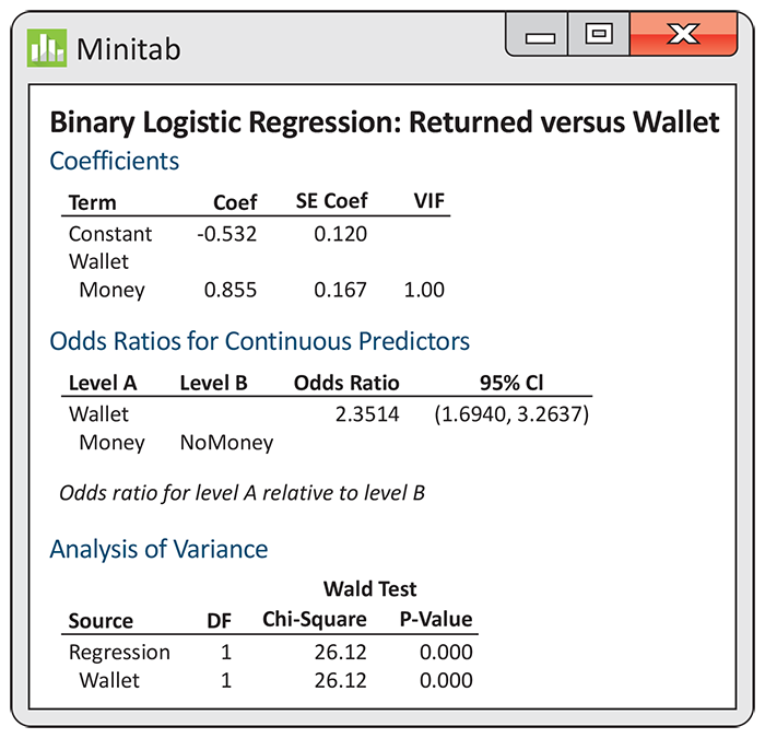
Figure 14.5 Minitab logistic regression output for the lost wallets example, Example 14.10.
The output also provides the odds ratio 2.3514 and a 95%
confidence interval, 1.6940 to 3.2637. Here is an interpretation of
the results in terms of odds: “The odds that wallets with money are
returned are more than twice the odds that wallets with no money are
returned
Check-in
-
14.9 Verify the calculation of the odds ratio. Refer to Check-in question 14.7. Verify that the odds ratio, 2.3514, is
-
14.10 Verify the calculation of the confidence interval. Refer to Example 14.10. Verify that the 95% confidence interval for the odds ratio, 1.69 to 3.26, can be transforming the 95% confidence interval for
where
In applications such as these, it is standard to use 95% confidence
for the odds ratio. This confidence interval gives us the result of
testing the null hypothesis that the odds ratio is 1 for a
significance level of 0.05. If the confidence interval does not
include 1, we reject
The following example is typical of many applications of logistic regression. Here, there is a designed experiment with five different values for the explanatory variable.
Example 14.11 An insecticide for aphids.
![]()

An experiment was designed to examine how well the insecticide rotenone kills an aphid, called Macrosiphoniella sanborni, that feeds on the chrysanthemum plant.4 The explanatory variable is the concentration (in log of milligrams per liter) of the insecticide. At each concentration, approximately 50 insects were exposed. Each insect was either killed or not killed. We summarize the data using the number killed at each concentration. Here are the data:
| Concentration (log(g/l)) | Number of insects | Number killed |
|---|---|---|
| 0.96 | 50 | 6 |
| 1.33 | 48 | 16 |
| 1.63 | 46 | 24 |
| 2.04 | 49 | 42 |
| 2.32 | 50 | 44 |
Because there are multiple insect trials at each concentration, we can estimate the proportion and log odds at each concentration. The logistic regression model assumes the log odds are linearly related to concentration so we can assess that here using a scatterplot with the least squares fit of a straight line (Figure 14.6). The linear fit is good.
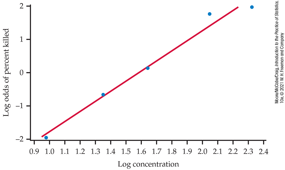
Figure 14.6 Plot of log odds of percent killed versus log concentration for the insecticide data, Example 14.11.
If we transform the response variable (by taking log odds) and use least squares, we get the fit illustrated in Figure 14.6. The logistic regression fit is given in Figure 14.7. It is a transformed version of Figure 14.6 with the fit calculated using the logistic model.
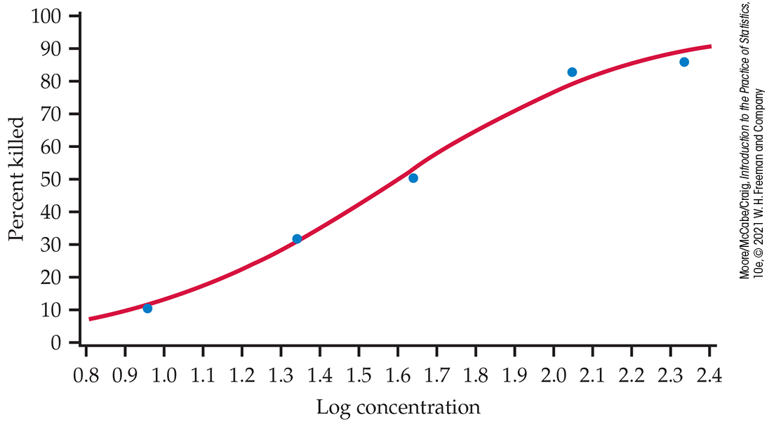
Figure 14.7 Plot of the percent killed versus log concentration with the logistic fit for the insecticide data, Example 14.11.
One of the major themes of this text is that we should present the
results of a statistical analysis with a graph. For the insecticide
example, we have done this with
Figure 14.7, and
the results appear to be convincing. But suppose that rotenone has no
ability to kill Macrosiphoniella sanborni. What is the chance
that we would observe experimental results at least as convincing to
what we observed if this supposition were true? The answer is the
P-value for the test of the null hypothesis that the logistic
regression coefficient
Example 14.12 Inference for aphid insecticide.
![]()
Figure 14.8 gives the output from Minitab, SPSS, and JMP for the logistic regression analysis of the insecticide data. The model is
where the values of the explanatory variable log of the insecticide concentration (x) are 0.96, 1.33, 1.63, 2.04, and 2.32. From the output in Minitab and SPSS, we see that the fitted model is
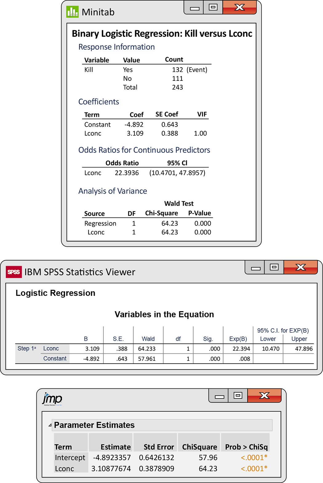
Figure 14.8 Logistic regression outputs from Minitab, SPSS, and JMP for the insecticide data, Example 14.12.
This is the fit transformed to percent killed that we plotted in
Figure 14.7.
The null hypothesis that
We are 95% confident that the true value of
The odds ratio is given in the Minitab output as 22.39. An increase
of one unit in the log concentration of insecticide (x) is
associated with a 22-fold
increase in the odds that an insect will be killed. Minitab gives
the 95% confidence interval for the odds ratio, 10.47 to 47.90. We
could calculate this from the confidence interval for
Note again that the test of the null hypothesis that
In Example 14.9, we studied the problem of predicting whether or not a movie was going to make a profit using the log opening-weekend revenue as the explanatory variable. We now revisit this example and show how statistical inference is an important part of the conclusion.
Example 14.13 Inference for movie profits.
![]()
Figure 14.9 gives the output from Minitab for a logistic regression analysis using log opening-weekend revenue (x) as the explanatory variable to predict the log odds that the movie will be profitable. From the Minitab output, we see that the fitted model is
In the output, the significance test results are given as
chi-squared statistics. We use the estimate
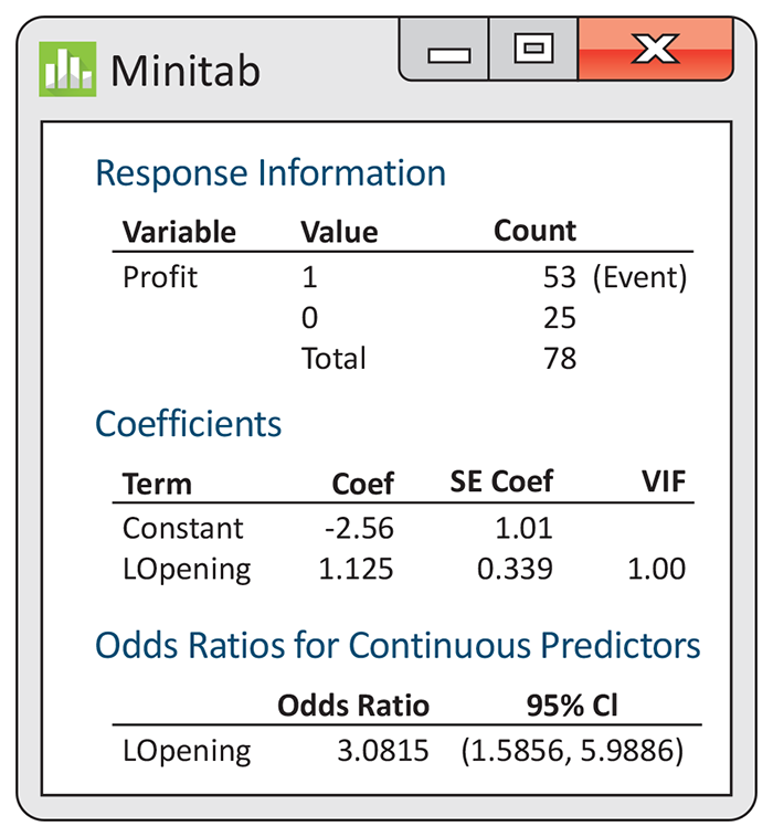
Figure 14.9 Minitab logistic regression output for the movie profitability data with log opening-weekend revenue as the explanatory variable, Example 14.13.
![]()
Our estimate of
We estimate that an opening-weekend revenue that is one unit larger (roughly $2.71 million) will increase the odds that a movie is profitable by about three times. The data, however, do not give us a very accurate estimate. The odds ratio could be as small as 1.6 or as large as 6.0 with 95% confidence. We have evidence to conclude that movies with higher opening-weekend revenues are more likely to be profitable, but establishing the relationship accurately would require more data.
Inference for multiple logistic regression
The movie example that we just considered naturally leads us to the next topic: inference for multiple logistic regression. The MOVIES data file includes additional explanatory variables. Do these other explanatory variables contain additional information that will give us a better prediction of profitability? Generating the computer output is easy, just as it was when we generalized simple linear regression with one explanatory variable to multiple linear regression with more than one explanatory variable in Chapter 11. The statistical concepts are similar, although the computations are more complex. Here is the example.
Example 14.14 Multiple logistic regression for movie profits.
![]()

As in Example 14.13, we predict the odds that a movie is profitable. The explanatory variables are log opening-weekend revenue (LOpening), number of theaters (Theaters), and a rating (Opinion) of the movie on a 1 to 10 scale (10 being best). Figure 14.10 gives the output from Minitab. The fitted model is
When analyzing data using multiple linear regression, we first examine the hypothesis that all the regression coefficients for the explanatory variables are zero. We do the same for multiple logistic regression. The hypothesis
is tested by a chi-square statistic with 3 degrees of freedom. (The
degrees of freedom are 3 because there are three coefficients that
are set to zero in the null hypothesis.) For Minitab, this is given
at the top of the Analysis of Variance output on the line titled
“Regression” under the label “Chi-square.” The value is 12.61, and
the P-value is given as 0.006. We reject
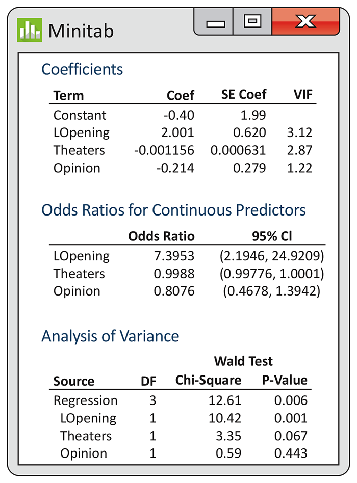
Figure 14.10 Minitab logistic regression output for the movie profitability data with log opening-weekend revenue, number of theaters, and movie’s rating as the explanatory variables, Example 14.14.
We now examine the coefficients for each variable and the tests that
each of these is zero in a model that contains the other two.
The P-values are 0.001, 0.067, and 0.443. The null hypotheses
Our initial multiple logistic regression analysis told us that the explanatory variables contain information that is useful for predicting whether or not the movie is profitable. Because the explanatory variables are correlated, however, we cannot clearly distinguish which variables or combinations of variables are important. Further analysis of these data using subsets of the three explanatory variables is needed to clarify the situation. See Exercise 14.37.
Section 14.2 SUMMARY
-
A level C confidence interval for
A level C confidence interval for the odds ratio
In these expressions, z* is the value for the standard Normal density curve with area C between
-
To test the hypothesis
and use the fact that z has a distribution that is approximately the standard Normal distribution when the null hypothesis is true. This statistic is sometimes called the Wald statistic. An alternative equivalent procedure is to report the square of z,
This statistic has a distribution that is approximately a
-
In multiple logistic regression the response variable has two possible values, as in logistic regression, but there can be k explanatory variables, where k can be greater than one. The null hypothesis that the regression coefficients for all explanatory variables are zero is tested by an
Section 14.2 EXERCISES
-
 14.13 Inference for teeth and military service.
Refer to
Exercise 14.4
(page 14-10), where you described a logistic regression model for a study
of whether U.S. recruits had enough teeth for adequate nutrition
during the Spanish–American War of 1898.
14.13 Inference for teeth and military service.
Refer to
Exercise 14.4
(page 14-10), where you described a logistic regression model for a study
of whether U.S. recruits had enough teeth for adequate nutrition
during the Spanish–American War of 1898.

-
Give the estimates of the regression parameters and write the equation of the fitted model.
-
Using the information provided in the output in Figure 14.4 (page 14-10), calculate and interpret the 95% confidence interval for the
-
Describe and interpret the results of the significance test for the regression coefficient
-
-
14.14 High blood pressure and cardiovascular disease. Refer to the study of cardiovascular disease and blood pressure in Exercise 14.6 (page 14-10). Computer output for a logistic regression analysis of these data gives the
-
Give a 95% confidence interval for
-
Calculate the
-
Write a short summary of your results and conclusions.
-
-
14.15 Odds ratio for teeth and military service. Refer to Exercise 14.13.
Give the odds ratio for this analysis.
-
Give the 95% confidence interval for the odds ratio.
-
Give a brief description of the meaning of the odds ratio in this analysis.
-
14.16 Odds ratio for high blood pressure and cardiovascular disease. The results describing the relationship between blood pressure and cardiovascular disease are given in terms of the change in log odds in Exercise 14.14.
-
Transform
-
Write a conclusion using the odds to describe the results.
-
-
14.17 What’s wrong? For each of the following, explain what is wrong and why.
-
For a multiple logistic regression with four explanatory variables, the null hypothesis that the regression coefficients of all the explanatory variables are zero is tested with an F test.
-
For a logistic regression, we assume that the model has a Normally distributed error term.
-
In logistic regression with one explanatory variable, we can use a chi-square statistic to test the null hypothesis
-
In multiple logistic regression, we do not need to worry about correlation among explanatory variables when interpreting model coefficient estimates.
-
-
14.18 Teeth and military service with six age categories. In Exercises 14.4, 14.13, and 14.15, we used logistic regression to study the relationship between being rejected for military service because a recruit did not have enough teeth and age, categorized into two groups, under 20 and 40 or over. Data are available for all recruits categorized into six age groups. Let’s look at a logistic regression that uses all the data to predict rejection for military service based on teeth. There are six age groups: under 20, 20–25, 25–30, 30–35, 35–40, and 40 or over. We define indicator explanatory variables for the last five groups. The first age group, under 20, will be zero for each of these indicator variables. This is similar to defining a single indicator explanatory variable for an analysis of two groups. Figure 14.11 gives the Minitab output for the logistic regression to predict rejection using the five age indicator explanatory variables.

Use the output to find the fitted model.
-
Is there a pattern in the values of the regression coefficients? If yes, describe it.
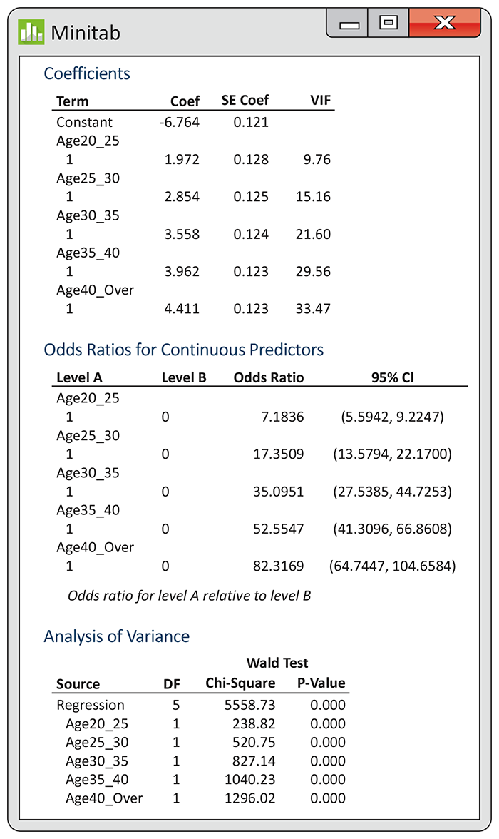
Figure 14.11 Minitab logistic regression output for predicting recruit rejection using age in six categories, for Exercises 14.18 through 14.20.
-
14.19 Inference for the multiple logistic regression model. Refer to the previous exercise.
-
Describe and interpret the significance test that tests the null hypothesis that all regression coefficients are zero.
-
Using the information provided in the output in Figure 14.11, calculate and interpret the 95% confidence interval for each of the regression coefficients.
-
Describe and interpret the results of the significance test for each regression coefficient. Be sure to give the null and alternative hypotheses, the test statistic, and the P-value with your conclusion.
-
-
14.20 Odds ratios for the multiple logistic regression model. Refer to the two previous exercises.
-
Give the odds ratio for each explanatory variable.
-
Give the 95% confidence interval for each odds ratio.
-
Give a brief description of the meaning of each odds ratio in this analysis.
-
-
14.21 Give a 99% confidence interval for

-
14.22 Give a 95% confidence interval for the odds ratio. Refer to Exercise 14.15 and the outputs for teeth and military service in Figure 14.4 (page 14-10). Using the estimate