15.2 The Wilcoxon Signed Rank Test
![]()
We use the one-sample t procedures for inference about the mean of one population or for inference about the mean difference in a matched pairs setting. The matched pairs setting is more important because good studies are generally comparative. We previously discussed the sign test for this setting. We now meet a nonparametric procedure that uses ranks.
Example 15.13 Storytelling and reading.
![]()

Refer to the study of early childhood education that asked kindergarten students to retell two fairy tales that had been read to them earlier in the week (see Exercise 15.2, page 15-14. The first (Story 1) had been read to them, and the second (Story 2) had been read and also illustrated with pictures. An expert listened to recordings of the children retelling each story and assigned a score for certain uses of language. Higher scores are better. Here are the data for the five kindergarten students in the low-progress group:8
| Child | 1 | 2 | 3 | 4 | 5 |
|---|---|---|---|---|---|
| Story 2 | 0.77 | 0.49 | 0.66 | 0.28 | 0.38 |
| Story 1 | 0.40 | 0.72 | 0.00 | 0.36 | 0.55 |
| Difference | 0.37 | 0.66 |
Do illustrations improve how the children retell a story?
Because this is a matched pairs design, we base our inference on the differences. The matched pairs t test gives
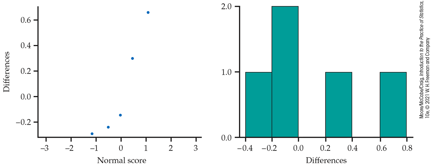
Figure 15.6 Normal quantile plot and histogram for the five differences in story scores, Example 15.13.
Example 15.14 Ranks for storytelling and reading.
![]()
Positive differences in Example 15.3 indicate that the child performed better telling Story 2. For the sign test, our test statistic was the number of positive differences. This ignored the size of the difference. We now use a test that also takes into account the size or magnitude. If scores are generally higher with illustrations, the positive differences should be farther from zero in the positive direction than the negative differences are in the negative direction. We, therefore, compare the absolute values of the differences—that is, their magnitudes without a sign. Here they are, with boldface indicating the positive values:
Arrange these in increasing order and assign ranks, keeping track of which values were originally positive. Tied values receive the average of their ranks. If there are cases with zero differences, discard them before ranking.
| Absolute value | 0.08 | 0.17 | 0.23 | 0.37 | 0.66 |
| Rank | 1 | 2 | 3 | 4 | 5 |
The ranks of the absolute values of the differences that are positive are also highlighted in bold face.
Now that we have ranks for both the positive and negative differences, we proceed in a manner similar to the Wilcoxon rank sum test. Here are the details of this test procedure.
Example 15.15 Wilcoxon signed rank statistic for storytelling and reading.
![]()
Here are the ranks for the absolute values of the differences in Example 15.14:
| Absolute value | 0.08 | 0.17 | 0.23 | 0.37 | 0.66 |
| Rank | 1 | 2 | 3 | 4 | 5 |
The Wilcoxon signed rank statistic is the sum of the ranks of the positive differences highlighted in bold. Its value here is
In this example, we have chosen to use the positive differences when summing the ranks. We could equally well use the sum of the ranks of the negative differences. In that case,
To determine the P-value, we need to know the null and alternative hypotheses.
Example 15.16 Storytelling and reading hypotheses.
Our question of interest is whether illustrations improve how children retell a story. Thus, we would like to test the null hypothesis
versus the alternative
The alternative hypothesis is a one-sided alternative, so now we can proceed to computing the P-value. In general, we will use software to either compute the exact P-value or approximate it using the Normal approximation.
Example 15.17 Software output.
![]()
In the storytelling study of Example 15.13, our observed value
Most statistical software uses the differences between the two variables, with the signs, as input. Alternatively, the differences can sometimes be calculated within the software. Figure 15.7 displays the output from three statistical programs. Each does things a little differently. The JMP output gives the one-sided (
Results reported in the three outputs lead us to the same qualitative conclusion: the data do not provide evidence to support the idea that the Story 2 scores are higher than (or not equal to) the Story 1 scores. Different methods and approximations are used to compute the P-values. With larger sample sizes, we would not expect so much variation in the P-values. Note that the t test results reported by JMP also gives the same conclusion,
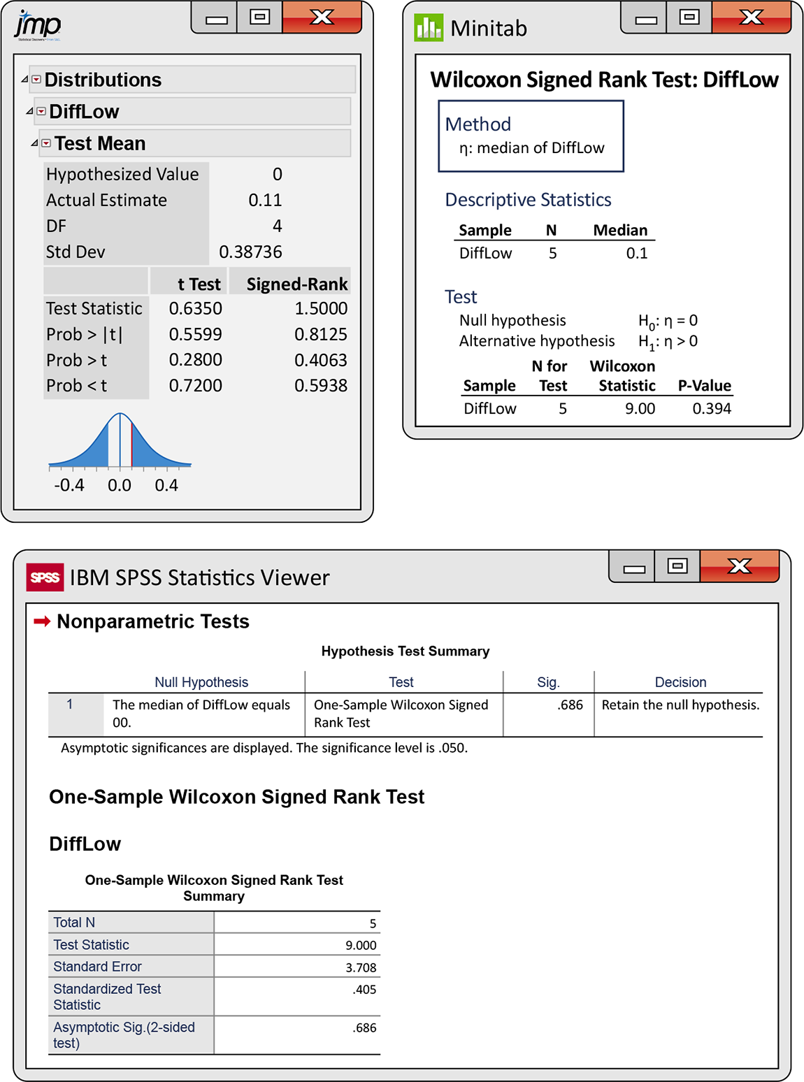
Figure 15.7 JMP, Minitab, and SPSS outputs for the storytelling data, Example 15.17.
When the sampling distribution of a test statistic is symmetric, we can use output that gives a P-value for a two-sided alternative to compute a P-value for a one-sided alternative. Check that the effect is in the direction specified by the one-sided alternative and then divide the P-value by 2.
Check-in
15.8 The effect of altering a software parameter. Example 7.7 (page 394) describes a study in which researchers studied sensor software used in the measurement of complex machine parts. They were interested in the possibility of improving productivity by unchecking one particular software option. They measured 76 parts both with and without the option. Use the data to investigate the effect of the option. Formulate this question in terms of null and alternative hypotheses. Then compute the differences and find the value of the Wilcoxon signed rank statistic

15.9 Cold plasma technology. Check-in question 7.10 (page 397) discusses a study related to the use of cold plasma (CP) technology for extending the shelf-life of food. For it to become widely used, however, CP’s effects on food quality must be understood. Consider the following study, which compared the taste of fruit juice with and without CP treatment. Each juice was rated by a set of taste experts, using a 0 to 100 scale, with 100 being the highest rating. For each expert, a coin was tossed to see which juice was tasted first.
Expert 1 2 3 4 5 6 7 8 9 10 With CP: 93 65 37 78 89 49 88 55 63 62 Without CP: 92 67 47 79 84 52 80 52 67 69 Use the the Wilcoxon signed rank test to examine whether the CP technology changes the taste of juice.

The Normal approximation
The distribution of the signed rank statistic when the null hypothesis (no difference) is true becomes approximately Normal as the sample size becomes large. We can then use Normal probability calculations (with the continuity correction) to obtain approximate P-values for
Example 15.18 The Normal approximation for storytelling and reading.
We first find the mean and the standard deviation for the distribution of
and the standard deviation is
Using the continuity correction, we calculate the P-value
Despite the small sample size, the Normal approximation gives a result quite close to the exact value
Check-in
15.10 Significance test for altering a software parameter. Refer to Check-in question 15.8 (page 15-19). Find
15.11 Significance test for the plasma technology. Refer to Check-in question 15.9 (page 15-19). Find
Ties
Ties among the absolute differences are handled by assigning average ranks. A tie within a pair gives a difference of zero. The usual procedure is to simply drop such pairs from the sample. A consequence of this convention is to drop observations that favor the null hypothesis (no difference). ![]() If there are many ties, the test may be biased in favor of the alternative hypothesis.
If there are many ties, the test may be biased in favor of the alternative hypothesis.
As in the case of the Wilcoxon rank sum procedure, ties between nonzero absolute differences complicate the process of finding a P-value. The standard deviation
Example 15.19 Golf scores of a women’s golf team.
![]()

Here are the golf scores of 12 members of a college women’s golf team in two rounds of tournament play. A golf score is the number of strokes required to complete the course, so low scores are better.
| Player | 1 | 2 | 3 | 4 | 5 | 6 | 7 | 8 | 9 | 10 | 11 | 12 |
|---|---|---|---|---|---|---|---|---|---|---|---|---|
| Round 2 | 94 | 85 | 89 | 89 | 81 | 76 | 107 | 89 | 87 | 91 | 88 | 80 |
| Round 1 | 89 | 90 | 87 | 95 | 86 | 81 | 102 | 105 | 83 | 88 | 91 | 79 |
| Difference | 5 | 2 | 5 | 4 | 3 | 1 |
Because we subtract Round 1 scores from Round 2 scores, negative differences indicate better (lower) scores on the second round. We see that 6 of the 12 golfers improved their scores. We would like to test the hypotheses that in a large population of collegiate women golfers
A Normal quantile plot of the differences (Figure 15.8) shows some irregularity and a low outlier. We will use the Wilcoxon signed rank test. The absolute values of the differences, with boldface indicating those that are negative, are
Arrange these in increasing order and assign ranks, keeping track of which values were originally negative. Tied values receive the average of their ranks.
| Absolute value | 1 | 2 | 3 | 3 | 4 | 5 | 5 | 5 | 5 | 5 | 6 | 16 |
| Rank | 1 | 2 | 3.5 | 3.5 | 5 | 8 | 8 | 8 | 8 | 8 | 11 | 12 |
The Wilcoxon signed rank statistic is the sum of the ranks of the negative differences. (We could equally well use the sum of the ranks of the positive differences.) Its value is
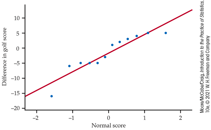
Figure 15.8 Normal quantile plot of the difference in scores for two rounds of a golf tournament, Example 15.19.
Example 15.20 Software output for P-values.
![]()
Here are the two-sided P-values for the Wilcoxon signed rank test for the golf score data from three statistical programs:
| Program | P-value |
|---|---|
| JMP | |
| Minitab | |
| SPSS |
All lead to the same practical conclusion: these data give no evidence for a systematic change in scores between rounds. However, the P-value reported by SPSS differs a bit from the other two. The reason for the variation is that the programs use slightly different versions of the approximate calculations needed when ties are present. The reported P-value depends on which version is used.
For the golf data, the matched pairs t test gives
Testing a hypothesis about the median of a distribution
Let’s take another look at how the Wilcoxon signed rank test works. The analysis starts by computing the differences between the two variables. At this stage, we can think of our data as consisting of a single variable. Under the null hypothesis, the population median of the differences is zero. The alternative is that the median is not zero. Now think about starting the analysis at the stage with just a single variable and keep in mind that we are interested in testing a hypothesis about the median of the variable’s distribution.
The value specified by the null hypothesis does not need to be zero. If you can’t specify a value other than zero with your software, you can simply subtract that value from each observation before you start the analysis. Exercise 15.14 is an example.
Section 15.2 SUMMARY
The Wilcoxon signed rank test applies to matched pairs studies. It tests the null hypothesis that there is no systematic difference within pairs against alternatives that assert a systematic difference (either one-sided or two-sided).
The test is based on the Wilcoxon signed rank statistic
P-values for the signed rank test are based on the sampling distribution of
Section 15.2 EXERCISES
15.13 Fuel efficiency. Computers in some vehicles calculate various quantities related to performance. One of these is the fuel efficiency, or gas mileage, usually expressed as miles per gallon (mpg). For one vehicle equipped in this way, the driver recorded the vehicle’s mpg each time the gas tank was filled and then reset the computer. In addition to the computer calculating mpg, the driver also recorded the mpg by dividing the miles driven by the number of gallons at fill-up.9 The driver wants to determine if these calculations are different.

Fill-up 1 2 3 4 5 6 7 Computer 42.2 43.2 44.6 48.4 46.4 46.8 39.2 Driver 39.2 38.8 44.5 45.4 45.3 45.7 34.2 For each of the eight fill-ups, find the difference between the computer mpg and the driver mpg.
Find the absolute values of the differences you found in part (a).
Order the absolute values of the differences that you found in part (b) from smallest to largest and underline those absolute differences that came from positive differences in part (a).
15.14 Comparison of two energy drinks. Consider the following study comparing two popular energy drinks. For each subject, a coin was flipped to determine which drink to rate first. Each drink was rated on a 0 to 100 scale, with 100 being the highest rating.

Drink Subject 1 2 3 4 5 6 A 43 83 66 87 78 67 B 45 78 64 79 71 62 Inspect the data. Is there a tendency for these subjects to prefer one of the two energy drinks?
Use the matched pairs t test from Chapter 7 (page 393) to compare the two drinks.
Use the Wilcoxon signed rank test to compare the two drinks.
Write a summary of your results and explain why the two tests give different conclusions.
15.15 Find the Wilcoxon signed rank statistic. Using the work that you performed in Exercise 15.13, find the value of the Wilcoxon signed rank statistic
15.16 Number of friends on Facebook. A study examined all active Facebook users (more than 10% of the global population) and determined that the average user has 190 friends. This distribution takes only integer values, so it is certainly not Normal. It is also highly skewed to the right, with a median of 100 friends.10 Consider the following SRS of

594 60 417 120 132 176 516 319 734 8 31 325 52 63 537 27 368 11 12 190 85 165 288 65 57 81 257 24 297 148 Use the Wilcoxon signed rank test to test the null hypothesis that the median number of Facebook friends for Facebook users at your university is 190. Describe the steps in the procedure and summarize the results.
Analyze these data using the matched pairs t test of Chapter 7 (page 393) and compare the results with those that you found in part (a).
15.17 State the hypotheses. Refer to Exercise 15.13. State the null hypothesis and the alternative hypothesis for this setting.
15.18 Comparison of two energy drinks with an additional subject. Refer to Exercise 15.14. Let’s suppose that there is an additional subject who expresses a strong preference for energy drink B. Here is the new data set:

Drink Subject 1 2 3 4 5 6 7 A 43 83 66 87 78 67 90 B 45 78 64 79 71 62 60 Answer the questions given in Exercise 15.14. Write a summary comparing this exercise with Exercise 15.14. Include a discussion of what you have learned regarding the choice of the t test versus the Wilcoxon signed rank test for different sets of data.
15.19 Find the mean and the standard deviation. Refer to the odd-numbered exercises from Exercise 15.13 through Exercise 15.17. Use the sample size to find the mean and the standard deviation of the sampling distribution of the Wilcoxon signed rank statistic
15.20 A summer language institute for teachers. A matched pairs study of the effect of a summer language institute on the ability of teachers to comprehend spoken French had these improvements in scores between the pretest and the posttest for 20 teachers:

2 0 6 6 3 3 2 3 6 6 6 3 0 1 1 0 2 3 3 Show how you rank these data.
Calculate the signed rank statistic
Perform the significance test and write a short summary of your conclusions.
15.21 Find and interpret the P-value. Refer to the odd-numbered exercises from Exercise 15.13 through Exercise 15.19. Find the P-value for the Wilcoxon signed rank statistic using the Normal approximation with the continuity correction.
15.22 Read the output. The data in Exercise 15.13 are a subset of a larger set of data. Figure 15.9 gives Minitab output for the analysis of this larger set of data.

How many pairs of observations are in the larger data set?
What is the value of the Wilcoxon signed rank statistic
Report the P-value for the significance test and give a brief statement of your conclusion.
The output reports an estimated median. Explain how this statistic is calculated from the data.
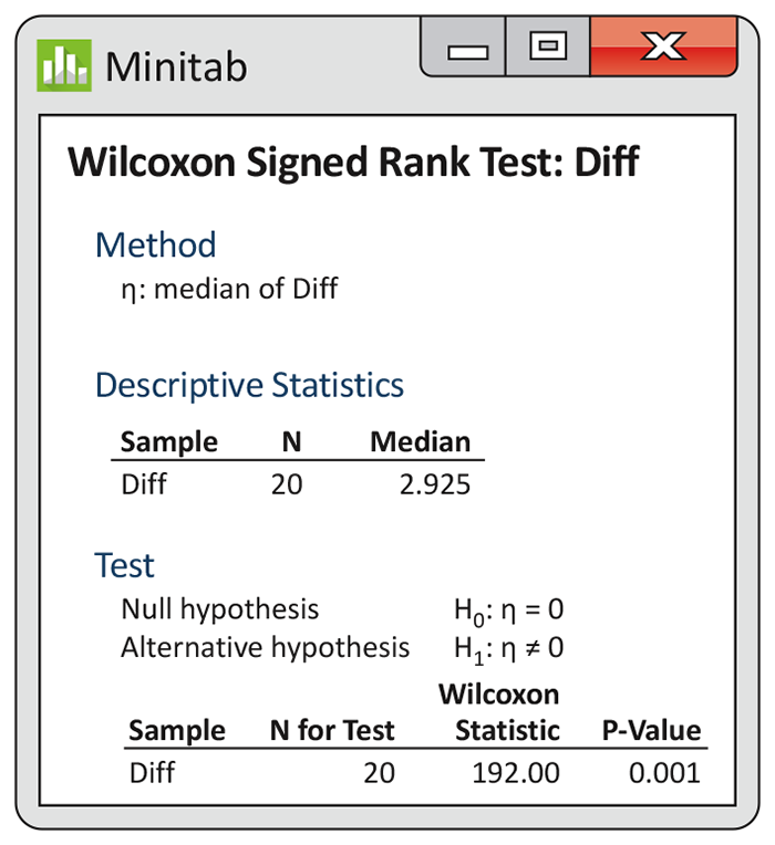
Figure 15.9 Minitab output for the fuel efficiency data, Exercise 15.22.
15.23 The full moon and behavior. Can the full moon influence behavior? A study observed 15 nursing-home patients with dementia. The number of incidents of aggressive behavior was recorded each day for 12 weeks. Here we call a day a “moon day” if it is the day of a full moon or the day before or after a full moon. Here are the average numbers of aggressive incidents for moon days and other days for each subject:11

Patient Moon days Other days 1 3.33 0.27 2 3.67 0.59 3 2.67 0.32 4 3.33 0.19 5 3.33 1.26 6 3.67 0.11 7 4.67 0.30 8 2.67 0.40 9 6.00 1.59 10 4.33 0.60 11 3.33 0.65 12 0.67 0.69 13 1.33 1.26 14 0.33 0.23 15 2.00 0.38 The matched pairs t test gives
 15.24 Radon detectors. How accurate are radon detectors of a type sold to homeowners? To answer this question, university researchers placed 12 detectors in a chamber that exposed them to 105 picocuries per liter (pCi/l) of radon.12 The detector readings are as follows:
91.9 97.8 111.4 122.3 105.4 95.0 103.8 99.6 96.6 119.3 104.8 101.7 We wonder if the median reading differs significantly from the true value 105.
Graph the data and comment on skewness and outliers. A rank test is appropriate.
We would like to test hypotheses about the median reading from home radon detectors:
To do this, apply the Wilcoxon signed rank statistic to the differences between the observations and 105. (This is the one-sample version of the test.) What do you conclude?
15.25 Vitamin C in wheat-soy blend. The U.S. Agency for International Development provides large quantities of wheat-soy blend (WSB) for development programs and emergency relief in countries throughout the world. One study collected data on the vitamin C content of five bags of WSB at the factory and five months later in Haiti.13 Here are the data:

Sample 1 2 3 4 5 Before 73 79 86 88 78 After 20 27 29 36 17
We want to know if vitamin C has been lost during transportation and storage. Describe what the data show about this question. Then use the Wilcoxon signed rank test to see whether there has been a significant loss.