5.3 Sampling Distributions for Counts and Proportions
In the previous section, we discussed the probability distribution of the sample mean, which involved focusing on quantitative population values. We will now shift our focus to population values that are categorical. Counts and proportions are common discrete statistics that describe categorical data.
We’ll focus on the setting when the categorical random variable has only two possible outcomes. In such situations, we can summarize the results by giving the count for one of the possible outcomes. We let n represent the sample size, and we use X to represent the count.
Example 5.15 Fact versus opinion.
The Programme for International Student Assessment (PISA) measures
15-year-olds’ abilities in reading, mathematics, and science
knowledge.13
Attaining a Level 5 or 6 score in the science knowledge portion means
the 15-year-old can distinguish fact from opinion through cues in the
material content, such as its sources. In the most recent assessment,
a total of
We would like to view the results of these
In our example, we chose X to be the number of U.S. 15-year-olds who attained a Level 5 or 6 science score. We could have chosen X to be the number of 15-year-olds who did not attain a Level 5 or 6 science score. Often, we make such a choice based on how we would like to describe the results in a summary.
Example 5.16 The sample proportion.
Rather than report X, it is more common to use the sample proportion as the summary. The sample proportion of U.S. 15-year-olds who attain a Level 5 or 6 science score is
Notice that the sample proportion takes into account the sample size
n. We need to know n in order to properly interpret the
meaning of the random variable X. For example, the conclusion we
would draw about U.S. 15-year-olds would be quite different if we had
observed
Check-in
-
5.14 Disapprove of trying marijuana. A survey of 2267 18-year-olds reports that 938 of them disapprove of people who are 18 or older trying marijuana.14 Give the sample size n, the count X, and the sample proportion
-
5.15 Use of the Internet to find a place to live. A poll of 1240 college students asked whether or not they used the Internet to find their current place to live. There were 904 students who answered Yes; the other 336 answered No.
-
What is the sample size n?
-
Choose one of the two possible outcomes to define the random variable X. Give a reason for your choice.
-
What is the value of the count X?
-
Find the sample proportion
-
Just like sample means, sample counts and sample proportions are commonly used statistics, and understanding their sampling distributions is important for statistical inference. These statistics, however, are discrete random variables, so their sampling distributions introduce us to two new families of probability distributions: the binomial and Poisson distributions.
In Section 5.1 (pages 273–275), we discussed the use of simulation to study the sampling distribution of the sample proportion. In this section, we will use probability theory to more precisely describe the sampling distributions of the sample count and proportion.
The binomial distributions for sample counts
The sampling distribution of any statistic depends on how the data are produced. Here is a simple but common situation for the count X.
Think of tossing a coin n times as an example of the binomial setting. Each toss, or observation, is either heads or tails, and the outcomes of successive tosses are independent. That is, knowing the result of one toss tells you nothing about the outcome of the following toss. If we call heads a success, then p is the probability of a head and remains the same as long as we toss the same coin. The number of heads we count is a random variable X. The distribution of X (and, more generally, the distribution of the count of successes in any binomial setting) is completely determined by the number of observations n and the success probability p.
The binomial distributions are an important class of discrete
probability distributions. We will soon learn how to assign
probabilities to outcomes and how to find the mean and standard
deviation of a binomial distribution.
![]() The most important skill for using binomial distributions, however,
is the ability to recognize situations to which they do and do not
apply.
This can be done by checking all the facets of the binomial setting.
The most important skill for using binomial distributions, however,
is the ability to recognize situations to which they do and do not
apply.
This can be done by checking all the facets of the binomial setting.
Example 5.17 Binomial examples?
-
Genetics says that children receive genes from their parents independently. Each child of a particular pair of parents has probability 0.25 of having type O blood. If these parents have three children, the number who have type O blood is the count X of successes in three independent trials with probability 0.25 of a success on each trial. So X has the B(3, 0.25) distribution.
-
Engineers define reliability as the probability that an item will perform its function under specific conditions for a specific period of time. Replacement heart valves made of animal tissue, for example, have probability 0.77 of performing well for 15 years.15 The probability of failure within 15 years is, therefore, 0.23. It is reasonable to assume that valves in different patients fail (or not) independently of each other. The number of patients in a group of 500 who will need another valve replacement within 15 years has the B(500, 0.23) distribution.
-
A multicenter trial is designed to assess a new surgical procedure. A total of 540 patients will undergo the procedure, and the count of patients X who suffer a major adverse cardiac event (MACE) within 30 days of surgery will be recorded. Because these patients will receive this procedure from different surgeons at different hospitals, it may not be true that the probability of a MACE is the same for each patient. Thus, X may not have the binomial distribution.
Check-in
-
5.16 Genetics and blood types. Genetics says that children receive genes from each of their parents independently. Suppose that each child of a particular pair of parents has probability 0.5625 of having type AB blood. If these parents have four children, what is the distribution of the number who have type AB blood? Explain your answer.
-
5.17 Tossing a coin. Suppose you plan to toss a coin 35 times and record X, the number of heads that you observe. If the coin is fair
Binomial distributions in statistical sampling
The binomial distributions are important in statistics when we wish to make inferences about the proportion p of “successes” in a population. Here is a typical example.
Example 5.18 Audits of financial records.

The financial records of businesses are often audited by state tax authorities to test compliance with tax laws. Suppose that for one retail business, 800 of the 10,000 sales are incorrectly classified as subject to state sales tax. It would be too time-consuming for authorities to examine all 10,000 sales. Instead, an auditor examines an SRS of sales records. Does the count X of misclassified records in an SRS of 150 records have the binomial distribution?
Choosing an SRS from a population is not quite a binomial setting. Removing one record changes the proportion of bad records in the remaining population, so the state of the second record chosen is not independent of the first. Because the population is large, however, removing a few items has a very small effect on the composition of the remaining population. Successive inspection results are very nearly independent. The population proportion of misclassified records is
If the first record chosen is bad, the proportion of bad records
remaining is
Populations like the one described in Example 5.18 often contain a relatively small number of cases with very large values. For this example, these cases could be records with very large sales amounts, an important group to the auditor. An SRS taken from the population will likely include very few records of this type. Therefore, it is common to use a stratified sample in settings like this. Strata are defined based on dollar value of the sale, and within each stratum, an SRS is taken. The results are then combined to obtain an estimate for the entire population.
Finding binomial probabilities
![]()
The formula for the probability that a binomial random variable takes any of its values is given in a later subsection. In practice, you will rarely have to use this formula for calculations because most calculators and statistical software packages can calculate binomial probabilities for you.
Example 5.19 Probabilities for misclassified sales records.
In the audit setting of Example 5.18, what is the probability that the audit finds exactly 10 misclassified sales records? What is the probability that the audit finds no more than 10 misclassified records? Figure 5.14 shows the output from one statistical software. You see that if the count X has the B(150, 0.08) distribution,
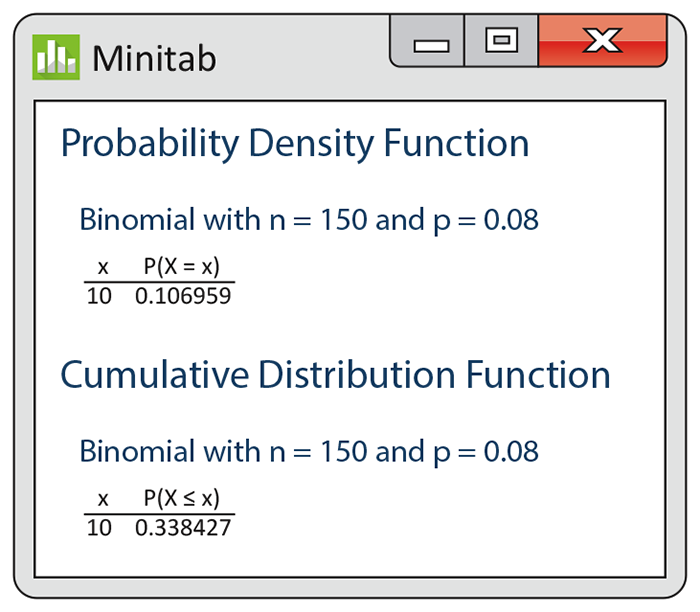
Figure 5.14 Minitab output of binomial probabilities, Example 5.19.
It is easy to request these calculations in the software’s menus.
For the TI-83/84 calculator, the functions
If you do not have suitable computing facilities, you can still
shorten the work of calculating binomial probabilities for some values
of n and p by looking up probabilities in
Table C
in the back of this book. The entries in the table are the
probabilities
Example 5.20 The probability histogram.
Suppose that the audit in Example 5.18 chose just 15 sales records. What is the probability that no more than 1 of the 15 is misclassified? The count X of misclassified records in the sample has approximately the B(15, 0.08) distribution. Figure 5.15 is a probability histogram for this distribution. The distribution is strongly skewed. Although X can take any whole-number value from 0 to 15, the probabilities of values larger than 5 are so small that they cannot be seen in the figure.
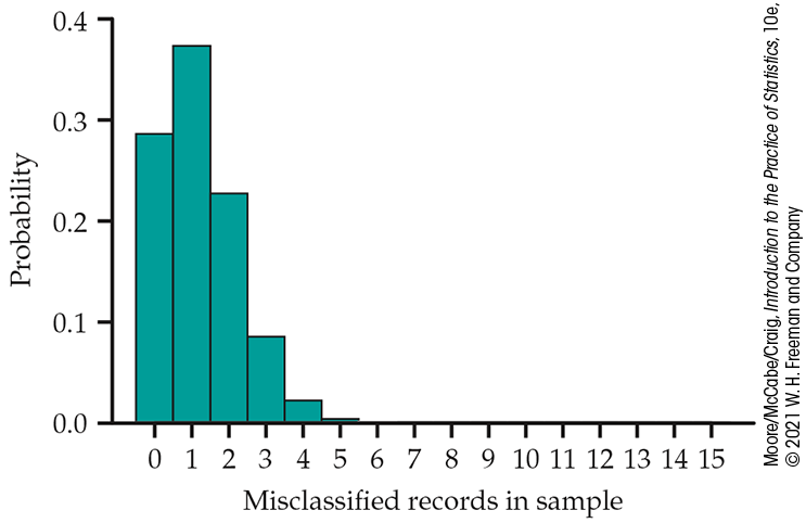
Figure 5.15
Probability histogram for the binomial distribution with
We want to calculate
when X has the B(15, 0.08) distribution. To use
Table C
for this calculation, look opposite
About two-thirds of all samples will contain no more than one bad record. In fact, almost 29% of the samples will contain no bad records. The sample of size 15 cannot be trusted to provide adequate evidence about misclassified sales records. A larger number of observations is needed.
| p | ||
|---|---|---|
| n | k | .08 |
| 15 | 0 | .2863 |
| 1 | .3734 | |
| 2 | .2273 | |
| 3 | .0857 | |
| 4 | .0223 | |
| 5 | .0043 | |
| 6 | .0006 | |
| 7 | .0001 | |
| 8 | ||
| 9 |
The values of p that appear in Table C are all 0.5 or smaller. When the probability of a success is greater than 0.5, restate the problem in terms of the number of failures. The probability of a failure is less than 0.5 when the probability of a success exceeds 0.5. When using the table, always stop to ask whether you must count successes or failures.
Example 5.21 Prevalence of vaping among high school seniors.
In a survey of 4583 high school seniors, 25% of the respondents reported nicotine vaping in the past 30 days.16 You randomly sample 10 students in your dormitory, and 6 state that they nicotine vaped in the past 30 days. Relative to the survey results, is this an unusually high number of students?
To answer this question, assume that the students’ actions (vaping or not) are independent, with the probability of nicotine vaping equal to 0.25. This independence assumption may not be reasonable if the students study and socialize together. We’ll assume this is not an issue here, so the number X of students who nicotine vaped out of 10 students has the B(10, 0.25) distribution.
We want the probability of classifying at least 6 students as having vaped in the past 30 days. Using Table C, we find
We would expect to find 6 or more students having vaped in the past
30 days about 2% of the time or in fewer than 1 of every 50 surveys
of 10 students. This is a pretty rare outcome if
Check-in
-
5.18 Free-throw shooting. Karissa is a college basketball player who makes 85% of her free throws. In a recent game, she had 7 free throws and missed 3 of them. Using software, a calculator, or Table C, compute
-
5.19 Find the probabilities.
-
Suppose that X has the B(9, 0.3) distribution. Use software, a calculator, or Table C to find
-
Suppose that X has the B(9, 0.7) distribution. Use software, a calculator, or Table C to find
-
Explain the relationship between your answers to parts (a) and (b) of this exercise.
-
Binomial mean and standard deviation
If a count X has the B(n, p) distribution,
what are the mean
Intuition suggests more generally that the mean of the B(n, p) distribution should be np. In fact, we can show that this is correct and also obtain a short formula for the standard deviation by using probability theory. We can use the mean and variance definitions of a discrete random variable or we can use the properties of a binomial random variable. The latter is much easier.
A binomial random variable X is the count of successes in
n independent observations that each have the same probability
p of success. Let the random variable
| Outcome | 1 | 0 |
| Probability | p |
|
From the definition of the mean of a discrete random variable, we know
that the mean of each
Similarly, the definition of the variance shows that
Because each
Apply the addition rules for means and variances to this sum. To find
the mean of X we add the means of the
Similarly, the variance is n times the variance of a single
S, so that
Notice that both the mean and the variance of a count
X increase with n. This will not be the case for
Example 5.22 The Helsinki Heart Study.
The Helsinki Heart Study asked whether the anticholesterol drug gemfibrozil reduces heart attacks. In planning such an experiment, the researchers must be confident that the sample sizes are large enough to enable them to observe enough heart attacks. The Helsinki study planned to give gemfibrozil to about 2000 men aged 40 to 55 and a placebo to another 2000. The probability of a heart attack during the five-year period of the study for men this age is about 0.04. What are the mean and standard deviation of the number of heart attacks that will be observed in one group if the treatment does not change this probability?
There are 2000 independent observations, each having probability
The expected number of heart attacks is large enough to permit
conclusions about the effectiveness of the drug. In fact, there were
84 heart attacks among the 2035 men actually assigned to the
placebo, quite close to the mean. The gemfibrozil group of 2046 men
suffered only 56 heart attacks. This is evidence that the drug
reduces the chance of a heart attack. In fact, software tells us
Check-in
-
5.20 Free-throw shooting. Refer to Check-in question 5.18. If Karissa takes 94 free throws in the upcoming season, what are the mean and standard deviation of the number of free throws made?
-
5.21 Find the mean and standard deviation.
-
Suppose that X has the B(9, 0.3) distribution. Compute the mean and standard deviation of X.
-
Suppose that X has the B(9, 0.7) distribution. Compute the mean and standard deviation of X.
-
Explain the relationship between your answers to parts (a) and (b) of this exercise.
-
Sample proportions
What proportion of a company’s sales records have an incorrect sales tax classification? What percent of adults favor stricter background checks on gun sales? In statistical sampling, we often want to estimate the proportion p of “successes” in a population. Our estimator is the sample proportion of successes:
![]() Be sure to distinguish between the proportion
Be sure to distinguish between the proportion
Example 5.23 Shopping online.

A survey by the Consumer Reports National Research Center revealed that 84% of all respondents were very satisfied with their online shopping experience.17 It was also reported, however, that people over the age of 40 were generally more satisfied than younger respondents. You decide to take a nationwide random sample of 2500 college students and ask if they agree or disagree that “I am very satisfied with my online shopping experience.” Suppose that 60% of all college students would agree with this statement. What is the probability that the sample proportion who agree is at least 58%?
The count X who agree has the binomial distribution
B(2500, 0.6). The sample proportion
Using software, we find that
To do the calculation in Example 5.23 by hand would be very involved. We would have to calculate and add more than 1000 binomial probabilities; most of us would not consider this a fun task! So what do we do if we don’t have access to software? Are we just going to have to plod through this? Thankfully, the answer is No.
As a first step, find the mean and standard deviation of a sample proportion. We know the mean and standard deviation of a sample count, so apply the rules for the mean and variance of a constant times a random variable. Here is the result.
Let’s now use these formulas to calculate the mean and standard deviation for Example 5.23.
Example 5.24 The mean and the standard deviation.
The mean and standard deviation of the proportion of the survey respondents in Example 5.23 who are satisfied with their online shopping experience are
Check-in
-
5.22 Find the mean and the standard deviation. If we toss a fair coin 150 times, the number of heads is a random variable that is binomial.
-
Find the mean and the standard deviation of the sample proportion of heads.
-
Is your answer to part (a) the same as the mean and the standard deviation of the sample count of heads in 150 throws? Explain your answer.
-
The fact that the mean of
In the simulation experiment on
page 274 in
Section 5.1, we also observed that the variability of
Normal approximation for counts and proportions
Using simulation, we discovered in
Section 5.1
that the sampling distribution of a sample proportion
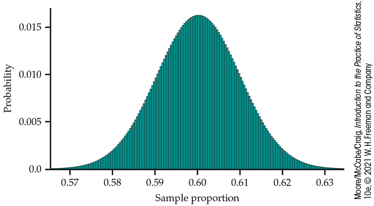
Figure 5.16 Probability
histogram of the sample proportion
We know this to be true as a result of the central limit theorem discussed in the previous section (page 287). Recall that we can consider the count X as a sum
of independent random variables
These Normal approximations are easy to remember because they say
that
![]() The accuracy of the Normal approximations improves as the sample size
n increases. They are most accurate for any fixed n when
p is close to 1/2, and they are least accurate when p is
near 0 or 1. You can compare binomial distributions with their Normal
approximations by using the
Normal Approximation to Binomial applet. This applet allows you
to change n or p while watching the effect on the
binomial probability histogram and the Normal curve that approximates
it.
The accuracy of the Normal approximations improves as the sample size
n increases. They are most accurate for any fixed n when
p is close to 1/2, and they are least accurate when p is
near 0 or 1. You can compare binomial distributions with their Normal
approximations by using the
Normal Approximation to Binomial applet. This applet allows you
to change n or p while watching the effect on the
binomial probability histogram and the Normal curve that approximates
it.
Figure 5.17 summarizes the distribution of a sample proportion in a form that emphasizes the big idea of a sampling distribution. Just as with Figure 5.11 (page 292), the general framework for constructing a sampling distribution is shown on the left and involves the following steps:
- Take many random samples of size n from a population that contains proportion p of successes.
-
Find the sample proportion
-
Collect all the
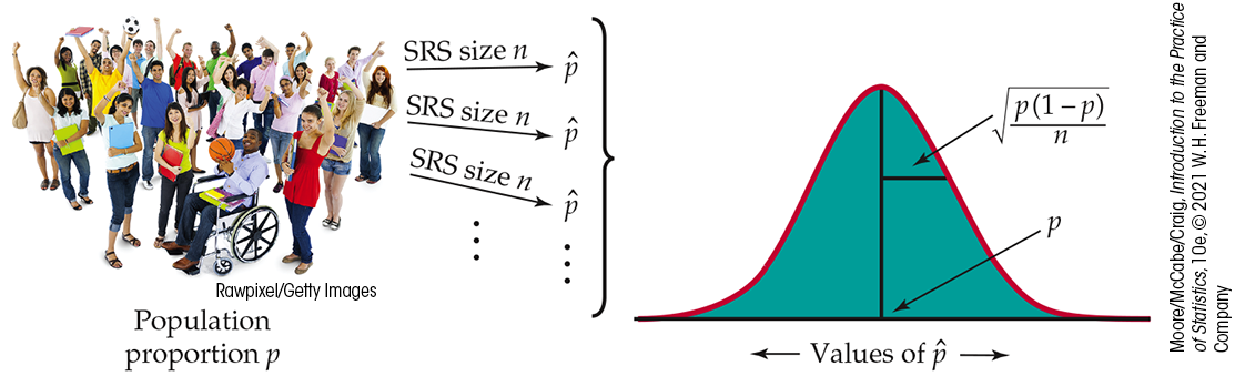
Figure 5.17 The
sampling distribution of a sample proportion
The sampling distribution of
Example 5.25 Compare the Normal approximation with the exact calculation.
Let’s compare the Normal approximation for the calculation of
Example 5.23 with the
exact calculation from software. We want to calculate
Act as if
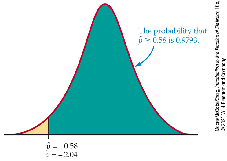
Figure 5.18 The Normal probability calculation, Example 5.25.
That is, about 98% of all samples have a sample proportion that is at least 0.58. Because the sample was large, this Normal approximation is quite accurate. It misses the software value 0.9802 by only 0.0009.
Example 5.26 Using the Normal approximation.
The audit described in Example 5.18 examined an SRS of 150 sales records for compliance with sales tax laws. In fact, 8% of all the company’s sales records have an incorrect sales tax classification. The count X of bad records in the sample has approximately the B(150, 0.08) distribution.
According to the Normal approximation to the binomial distributions, the count X is approximately Normal, with mean and standard deviation
The Normal approximation for the probability of no more than 10
misclassified records is the area to the left of
Software tells us that the actual binomial probability that no more
than 10 of the records in the sample are misclassified is
The distribution of the count of bad records in a sample of 15 is distinctly non-Normal, as Figure 5.15 (page 302) showed. When we increase the sample size to 150, however, the shape of the binomial distribution becomes roughly Normal. Figure 5.19 displays the probability histogram of the binomial distribution with the density curve of the approximating Normal distribution superimposed. The two distributions have the same mean and standard deviation, and both the area under the histogram and the area under the curve are 1. The Normal curve fits the histogram reasonably well. Look closely: the histogram is slightly skewed to the right, a property that the symmetric Normal curve can’t match.
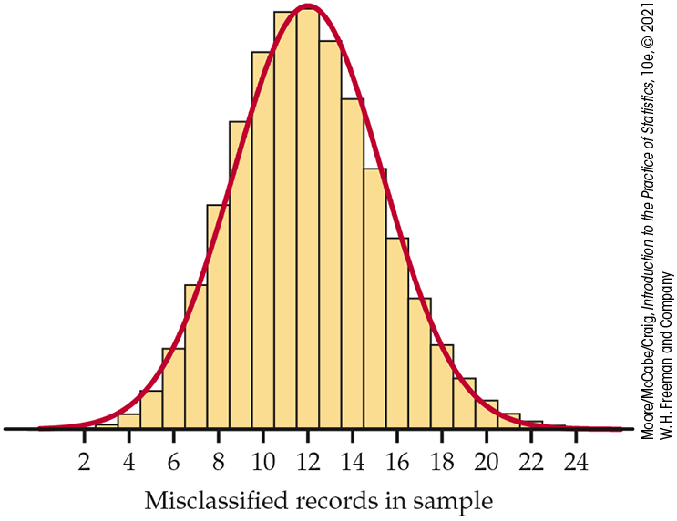
Figure 5.19 Probability
histogram and Normal approximation for the binomial distribution
with
Check-in
-
5.23 Use the Normal approximation. In Example 5.22, software told us
-
What are the mean and standard deviation of X?
-
Use the Normal approximation to find
-
The continuity correction
Figure 5.20
illustrates an idea that greatly improves the accuracy of the Normal
approximation to binomial probabilities. The binomial probability
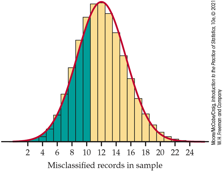
Figure 5.20 Area under the Normal approximation curve for the probability in Example 5.26.
The Normal approximation is more accurate if we consider
The improved approximation misses the binomial probability by only 0.012. Acting as though a whole number occupies the interval from 0.5 below to 0.5 above the number is called the continuity correction to the Normal approximation. If you need accurate values for binomial probabilities, try to use software to do exact calculations. If no software is available, use the continuity correction unless n is very large. Because most statistical purposes do not require extremely accurate probability calculations, we do not emphasize use of the continuity correction.
Binomial formula
We can find a formula for the probability that a binomial random variable takes any value by adding probabilities for the different ways of getting exactly that many successes in n observations. Here is the example we will use to show the idea.
Example 5.27 Blood types of children.
Each child born to a particular set of parents has probability 0.25 of having blood type O. If these parents have five children, what is the probability that exactly two of them have type O blood?
The count of children with type O blood is a binomial random
variable X with
Because the method doesn’t depend on the specific example, we will use “S” for success and “F” for failure. In Example 5.27, “S” would stand for type O blood. Do the work in two steps.
-
Step 1. Find the probability that a specific two of the five tries give successes—say, the first and the third. This is the outcome SFSFF. The multiplication rule for independent events tells us that
-
Step 2. Observe that the probability of any one arrangement of two S’s and three F’s has this same probability. That’s true because we multiply together 0.25 twice and 0.75 three times whenever we have two S’s and three F’s. The probability that
There are 10 of them, all with the same probability. The overall probability of two successes is, therefore,
The pattern of this calculation works for any binomial probability. To use it, we need to be able to count the number of arrangements of k successes in n observations without actually listing them. We use the following fact to do the counting.
The formula for binomial coefficients uses the factorial notation. The factorial n! for any positive whole number n is
Also,
This agrees with our previous calculation.
![]() The notation
The notation
Here is an example of the use of the binomial probability formula.
Example 5.28 Using the binomial probability formula.
The number X of misclassified sales records in the auditor’s sample in Example 5.20 (page 302) has the B(15, 0.08) distribution. The probability of finding no more than one misclassified record is
The calculation used the facts that
Check-in
-
5.24 An unfair coin. A coin is slightly bent, and as a result, the probability of a head is 0.55. Suppose that you toss the coin five times.
-
Use the binomial formula to find the probability of three or more heads.
-
Compare your answer with the one that you would obtain if the coin were fair.
-
The Poisson distributions for sample counts
A count X has a binomial distribution when it is produced under the binomial setting. If one or more facets of this setting do not hold, the count X will have a different distribution. In this subsection, we discuss one of these distributions.
Frequently, we meet counts that are open-ended; that is, they are not based on a fixed number of n observations: the number of customers at a popular café between 12:00 p.m. and 1:00 p.m.; the number of dings on your car door; the number of reported pedestrian/bicyclist collisions on campus during the academic year. These are all counts that could be 0, 1, 2, 3, and so on indefinitely.
The family of Poisson distributions is another model for a count and can often be used in these open-ended situations. The count represents the number of events (call them “successes”) that occur in some fixed unit of measure such as a period of time or region of space. The Poisson distribution is appropriate if the following conditions are met.
For binomial distributions, the important quantities were n,
the fixed number of observations, and p, the probability of
success on any given observation. For Poisson distributions, the only
important quantity is the mean number of successes
Example 5.29 Number of school Wi-Fi slowdowns.
Suppose that the number of Wi-Fi slowdowns at your school varies,
with an average of 3.7 per day. If we assume that the Poisson
setting is reasonable for this situation, we can model the daily
count of slowdowns X by using the Poisson distribution with
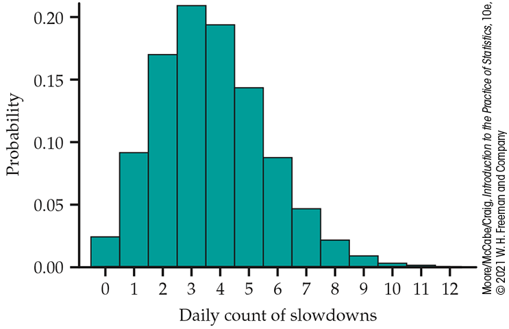
Figure 5.21
Probability histogram for the Poisson distribution with
We can calculate
Using the R software, the probability is
dpois(0, 3.7) + dpois(1, 3.7) + dpois(2, 3.7)
   [1]0.2854331
There is roughly a 29% chance that there will be no more than two Wi-Fi slowdowns tomorrow.
Much like binomial calculations, Poisson probability calculations
are rarely done by hand if the event includes numerous possible values
for X. Most software provides functions to calculate
Example 5.30 Counting software remote users.
Your university supplies online remote access to various software
programs used in courses. Suppose that the number of students
remotely accessing these programs in any given hour can be modeled
by a Poisson distribution with
Calculating this probability requires two steps.
-
Write
-
Obtain
1–ppois 25,17.2
[1] 0.02847261
The probability that more than 25 students will use this remote access in the next hour is only 0.028. Relying on software to get the cumulative probability is much quicker and less prone to error than the method of Example 5.29. For this case, that method would involve determining 26 probabilities and then summing their values.
Under the Poisson setting, this probability of 0.028 applies not only to the next hour but also to any other hour in the future. The probability does not change because the units of measure are the same size and nonoverlapping.
Check-in
-
5.25 Number of aphids. The milkweed aphid is a common pest to many ornamental plants. Suppose that the number of aphids on a shoot of a Mexican butterfly weed follows a Poisson distribution with
-
What is the probability of observing exactly 7 aphids on a shoot?
-
What is the probability of observing 5 or fewer aphids on a shoot?
-
-
5.26 Number of aphids, continued. Refer to the previous Check-in question.
-
What proportion of shoots would you expect to have no aphids present?
-
If you do not observe any aphids on a shoot, is the probability that a nearby shoot has no aphids smaller than, equal to, or larger than your answer in part (a)? Explain your reasoning.
-
If we add counts from successive nonoverlapping areas of equal size, we are just counting the successes in a larger area. That count still meets the conditions of the Poisson setting. However, because our unit of measure has doubled, the mean of this new count is twice as large. Put more formally:
This fact means that we can combine areas or look at a portion of an area and still use Poisson distributions to model the count.
Example 5.31 Number of potholes.

The Automobile Association (AA) in Britain had member volunteers make a 60-minute 2-mile walk around their neighborhoods and survey the condition of their roads and sidewalks. One outcome was the number of potholes, defined as being at least 2 inches deep and at least 6 inches in diameter, in their roads.18 It was reported that Scotland averages 8.9 potholes per mile of road and London averages 4.9 potholes per mile of road. Suppose that the number of potholes per mile in each of these two regions follow the Poisson distribution. Then
-
The number of potholes per 20 miles of road in Scotland is a
Poisson random variable with mean
-
The number of potholes per half mile of road in London is a
Poisson random variable with mean
-
The number of potholes per 500 miles of road in Scotland is a
Poisson random variable with mean
-
If we examined 2 miles of road in Scotland and 5 miles of road in
London, the total number of potholes would be a Poisson random
variable with mean
When the mean of the Poisson distribution is large, it may be
difficult to calculate Poisson probabilities using a calculator or
software. Fortunately, the central limit theorem says that when
Example 5.32 Number of snaps received.
In Example 5.11, it was reported that Snapchat has more than 200 million daily users sending well over 3 billion snaps a day. Suppose that the number of snaps you receive per day follows a Poisson distribution with mean 20. What is the probability that, over a week, you would receive more than 160 snaps?
To answer this question using software, we first compute the mean
number of snaps sent per week. Because there are seven days in a
week, the mean is
1 - ppois(160, 140)
 [1] 0.04396269
For the Normal approximation we compute
The approximation is quite accurate, differing from the actual probability by only 0.0015.
While the Normal approximation is adequate for many practical purposes, we recommend using statistical software when possible so you can get exact Poisson probabilities.
There is, however, one other approximation associated with the Poisson
distribution that is worth mentioning. It is related to the binomial
distribution. Previously, we recommended using the Normal distribution
to approximate the binomial distribution when n and
p satisfy
pbinom (2,1000,0.001) ppois (2,1)
[1] 0.9197907 [1]0.9196986
The Poisson approximation gives a very accurate probability calculation for the binomial distribution in this case.
Section 5.3 SUMMARY
-
A count X of successes has the binomial distribution B(n, p) in the binomial setting: there are n trials, all independent, each resulting in a success or a failure, and all having the same probability p of a success.
-
The binomial distribution B(n, p) is a good approximation to the sampling distribution of the count X of successes in an SRS of size n from a large population containing proportion p of successes. This approximation is adequate when the population is at least 20 times larger than the sample.
-
The sample proportion of successes
-
Binomial probabilities are most easily found by software. There is an exact formula that is practical for calculations when n is small. Table C contains binomial probabilities for some values of n and p. For large n, you can use the Normal approximation.
-
The mean and standard deviation of a binomial count X and a sample proportion
-
The Normal approximation to the binomial distribution says that if X is a count having the B(n, p) distribution, then when n is large,
This approximation is reasonably accurate when
-
The continuity correction improves the accuracy of the Normal approximations.
-
The exact binomial probability formula is
where the possible values of X are
which counts the number of ways of distributing k successes among n trials.
-
A count X of successes has a Poisson distribution in the Poisson setting: the numbers of successes that occur in two nonoverlapping units of measure are independent; the probability that a success will occur in a unit of measure is the same for all units of equal size and is proportional to the size of the unit; the probability that more than one event will occur in a unit of measure is negligible for very small-sized units. In other words, the events occur one at a time.
-
If X has the Poisson distribution with mean
-
The Poisson probability that X takes any of these values is
-
Sums of independent Poisson random variables also have the Poisson distribution. For example, in a Poisson model with mean
Section 5.3 EXERCISES
Most binomial probability calculations required in these exercises can be done by using Table C or the Normal approximation. Your instructor may request that you use the binomial probability formula or software. In exercises requiring the Normal approximation, use the continuity correction if you studied that topic. Poisson calculations can be done using software, the Poisson formula, or Normal approximation.
-
5.27 What’s wrong? For each of the following statements, explain what is wrong and why.
-
If you toss a fair coin four times and a head appears each time, then the next toss is more likely to be a head than a tail.
-
If you toss a fair coin four times and observe the pattern THTH, then the next toss is more likely to be a tail than a head.
-
The quantity
-
The binomial distribution can be used to model the daily number of pedestrian/cyclist near-crash events on campus.
-
-
5.28 What’s wrong? For each of the following statements, explain what is wrong and why.
-
In the binomial setting, X is a proportion.
-
The variance for a binomial count is
-
The Normal approximation to the binomial distribution is always accurate when n is very large.
-
The binomial distribution is a good approximation of the sampling distribution of the count X when we draw an SRS of size n students from a population of 5n students.
-
-
5.29 Should you use the binomial distribution? In each of the following situations, is it reasonable to use a binomial distribution for the random variable X? Give reasons for your answer in each case. If a binomial distribution applies, give the values of n and p.
-
A poll of 200 college students asks whether or not you usually feel irritable in the morning. X is the number who reply that they do usually feel irritable in the morning.
-
You toss a fair coin until a head appears. X is the count of the number of tosses that you make.
-
Most calls made at random by sample surveys don’t succeed in talking with a person. Of calls to New York City, only one-twelfth succeed. A survey calls 500 randomly selected numbers in New York City. X is the number of times that a person is reached.
-
You deal 10 cards from a shuffled deck of standard playing cards and count the number X of black cards.
-
-
5.30 Should you use the binomial distribution? In each of the following situations, is it reasonable to use a binomial distribution for the random variable X? Give reasons for your answer in each case.
-
In a random sample of students in a fitness study, X is the mean daily exercise time of the sample.
-
A manufacturer of running shoes picks a random sample of 20 shoes from the production of shoes each day for a detailed inspection. X is the number of pairs of shoes with a defect.
-
A nutrition study chooses an SRS of college students. They are asked whether or not they usually eat at least five servings of fruits or vegetables per day. X is the number who say that they do.
-
X is the number of days during the school year when you skip a class.
-
-
5.31 Random digits. Each entry in a table of random digits like Table B has probability 0.1 of being a 0, and digits are independent of each other.
-
What is the probability that a group of five digits from the table will contain at least one digit greater than 4?
-
What is the mean number of digits greater than 4 in lines 40 digits long?
-
-
5.32 Admitting students to college. A selective college would like to have an entering class of 900 students. Because not all students who are offered admission accept, the college admits more than 900 students. Past experience shows that about 78% of the students admitted will accept. The college decides to admit 1150 students. Assuming that students make their decisions independently, the number who accept has the B(1150, 0.78) distribution. If this number is less than 900, the college will admit students from its waiting list.
-
What are the mean and the standard deviation of the number X of students who accept?
-
The college does not want more than 900 students. Use the Normal approximation to find the probability that more than 900 students accept.
-
If the college decides to decrease the number of admission offers to 1100, what is the probability that more than 900 will accept?
-
Based on your answers to parts (b) and (c), should the college admit 1100 or 1150 students? Explain your answer.
-
-
5.33 Cyberbullying. A survey of 4972 U.S. students aged 12 to 17 years reveals that 25% have received mean or hurtful comments online in the past 30 days.19 You take a random sample of 15 undergraduates and ask them whether they have received mean or hurtful comments online in the past 30 days. If the rate at your university matches this 25% rate:
-
What is the distribution of the number of undergraduates who say that they have received hurtful comments online in the past 30 days?
-
What is the distribution of the number of undergraduates who say that they have not received hurtful comments online in the past 30 days?
-
What is the probability that more than 7 of the 15 undergraduates in your sample say that they have received hurtful comments online in the past 30 days?
-
What is the probability that no more than 7 of the 15 students in your sample say that they have not received hurtful comments online in the past 30 days?
-
-
5.34 Genetics of peas. According to genetic theory, the blossom color in the second generation of a certain cross of sweet peas should be red or white in a 3:1 ratio. That is, each plant has probability 3/4 of having red blossoms, and the blossom colors of separate plants are independent.
-
What is the probability that exactly 8 out of 10 of these plants have red blossoms?
-
What is the mean number of red-blossomed plants when 130 plants of this type are grown from seeds?
-
What is the probability of obtaining at least 90 red-blossomed plants when 130 plants are grown from seeds?
-
-
5.35 Cyberbullying, continued. Refer to Exercise 5.33.
-
What is the expected number of undergraduates in your sample who say that they have received hurtful comments online in the past 30 days? What is the expected number of undergraduates who say that they have not received hurtful comments online in the past 30 days? What do the two means add up to?
-
What is the standard deviation
-
What are the mean and standard deviation of
-
Repeat the calculations in parts (a)–(c) for a sample of
-
-
5.36 Online learning. The U.S. Department of Education released a report on online learning stating that blended instruction, a combination of conventional face-to-face and online instruction, appears to be more effective in terms of student performance than conventional teaching.20 You decide to poll incoming students at your institution to see if they prefer courses that blend face-to-face instruction with online components. In an SRS of 400 incoming students, you find that 373 prefer this type of course.
-
What is the sample proportion of incoming students at your school who prefer this type of blended instruction?
-
Assume that the population proportion for all students nationwide is 85%. Assuming that this is true for your institution too, what is the standard deviation of
-
Using the 68–95–99.7 rule, you would expect
-
Based on your result in part (a), do you think that the incoming students at your institution prefer this type of instruction more, less, or about the same as students nationally? Explain your answer.
-
-
5.37 Is the binomial distribution a reasonable approximation? In each of the following situations, is it reasonable to use a binomial distribution to approximate the sampling distribution of X? Give reasons for your answer in each case.
-
According to the Red Cross, 0.5% of the Asian ethnic group in the United States have type A– blood.21 Suppose that this national proportion holds for your large city. If you randomly sample 500 Asian residents, can the B(500, 0.005) distribution be used for the count X of Asian residents that have type A– blood?
-
You are interested in determining the proportion of residents on the Sci Fi floor at your university who binge watch Netflix at least once a week. There are a total of 50 residents on the floor. You choose 25 residents (1 per room) at random to interview. If the true proportion is 0.80, can the B(25, 0.80) distribution be used for the count X in your sample?
-
-
5.38 Mishandled bags. In the airline industry, the term mishandled refers to a bag that was lost, delayed, damaged, or stolen. The latest report by SITA states that the mishandled baggage rate has plateaued at 5.7 per 1000 passengers.22 Suppose that this national rate holds for your airport, and your airport typically has 10,000 passengers a month. Let X be the number of mishandled bags per month.
-
Do you think it is reasonable to use the Poisson distribution to model X? Explain your answer.
-
Using the Poisson distribution, what are the mean and standard deviation of X?
-
Use the Poisson approximation to find the probability that there will be more than 70 mishandled bags next month.
-
-
5.39 Shooting free throws. Since the mid-1960s, the overall free-throw percent at all college levels, for both men and women, has remained pretty consistent. For men, players have been successful on roughly 69% of free throws, with the season percent never falling below 67% or above 70%.23 Assume that 300,000 free throws will be attempted in the upcoming season.
-
What are the mean and standard deviation of
-
Using the 68–95–99.7 rule, we expect
-
Given the width of the interval in part (b) and the range of season percents, do you think that it is reasonable to assume that the population proportion has been the same over the last 50 seasons? Explain your answer.
-
-
 5.40 Show that these facts are true. Use the
definition of binomial coefficients to show that each of the
following facts is true. Then restate each fact in words in
terms of the number of ways that k successes can be
distributed among n observations.
5.40 Show that these facts are true. Use the
definition of binomial coefficients to show that each of the
following facts is true. Then restate each fact in words in
terms of the number of ways that k successes can be
distributed among n observations.
-
-
5.41 English Premier League goals. The total number of goals scored per soccer match in the English Premier League (EPL) often follows the Poisson distribution. In one recent season, the average number of goals scored per match (over 380 games played) was 2.821. Compute the following probabilities.
-
What is the probability that three or more goals will be scored in a game?
-
What is the probability that a game will end in a 0–0 tie?
-
What is the probability that a team will win
-
Explain why you cannot compute the probability that a game will end in a 1–1 tie but can provide an upper bound on this probability.
-
-
5.42 Number of colony-forming units. In microbiology, colony-forming units (CFUs) are used to measure the number of microorganisms present in a sample. To determine the number of CFUs, the sample is prepared, spread uniformly on an agar plate, and then incubated at some suitable temperature. Suppose that the number of CFUs that appear on the agar plate after incubation follows a Poisson distribution with
-
If the area of the agar plate is 75 square centimeters
-
If you were to count the total number of CFUs in five plates, what is the probability that you would observe more than 60 CFUs? Use the Poisson distribution to obtain this probability.
-
Repeat the probability calculation in part (b) but now use the Normal approximation. How close is your answer to your answer in part (b)?
-
-
5.43 Metal fatigue. Metal fatigue refers to the gradual weakening and eventual failure of metal that undergoes cyclic loads. The wings of an aircraft, for example, are subject to cyclic loads when in the air, and cracks can form. It is thought that these cracks start at large particles found in the metal. Suppose that the number of particles large enough to initiate a crack follows a Poisson distribution with mean
-
What is the mean of the Poisson distribution if we consider a 100
-
Using the Normal approximation, what is the probability that this section has more than 60 of these large particles?
-