8.1 Inference for a Single Proportion
We want to estimate the proportion p of some characteristic in a large population. For example, we may want to know the proportion of likely voters who approve of the president’s conduct in office. We select a simple random sample (SRS) of size n from the population and record the count X of “successes” (such as Yes answers to a question about the president). A “success” response represents the characteristic of interest in this example.
In statistical terms, we are concerned with inference about the
probability p of a success in the binomial setting. The sample
proportion of successes
Example 8.1 Robotics and jobs.
![]()
A Pew survey asked a panel of experts whether or not they thought that networked, automated, artificial intelligence (AI), and robotic devices will have displaced more jobs than they have created (net jobs) by 2025.2
The sample size is the number of experts who responded to the Pew
survey question,
Check-in
-
8.1 Users of Instagram. The Pew Research Center surveyed U.S. social media users. Among the 236 respondents who were 18 to 21 years old, 158 said that they used Instagram.3
-
What is the sample size n for the 18- to 21-year-olds?
-
In this setting, describe the population proportion p in a short sentence.
-
What is the count X? Describe the count in a short sentence.
-
Find the sample proportion
-
-
8.2 Users of Snapchat. Refer to the previous Check-in question. For the same 236 respondents, 62% said that they used Snapchat.
-
What is the sample size n for this setting?
-
What is the count X of those who said they use Snapchat?
-
What is the sample proportion
-
If the sample size n is very small, we must base tests and
confidence intervals for p on the binomial distributions. These
are awkward to work with because of the discreteness of the binomial
distributions.4
But we know that when the sample size n is large, both the count
X and the sample proportion
Large-sample confidence interval for a single proportion
The unknown population proportion p is estimated by the sample
proportion
Note that the standard deviation
Table D
at the back of the book includes a line at the bottom with values of
z* for selected values of C. Use
Table A
for other values of C. You can also use software, such as Excel
with the formula such as = NORM.S.INV(1−C).
Example 8.2 Inference for robotics and jobs.
![]()
The sample survey in Example 8.1 found that 910 of a sample of 1896 experts reported that they think net jobs will decrease by 2025 because of robots and related technology developments. The sample proportion is
which was rounded to 48% in their report. The standard error is
The z critical value for 95% confidence is
The confidence interval is
We are 95% confident that between 45.8% and 50.2% of experts would report that they think net jobs will decrease by 2025 because of robots and related technology developments.
In performing these calculations, we have kept a large number of
digits for our intermediate calculations to avoid rounding errors.
However, when reporting the results, we prefer to use rounded values
(for example, “48.0% with a margin of error of 2.2%”).
You should always focus on what is important.
![]() Reporting extra digits that are not needed can divert attention from
the main point of your summary.
There is no additional information to be gained by reporting
Reporting extra digits that are not needed can divert attention from
the main point of your summary.
There is no additional information to be gained by reporting
![]() Remember that the margin of error in any confidence interval
includes only random sampling error.
If people do not respond honestly to the questions asked, for example,
your estimate is likely to miss by more than the margin of error.
Likewise, if the response rate is low, your estimate and standard
error may be biased.
Remember that the margin of error in any confidence interval
includes only random sampling error.
If people do not respond honestly to the questions asked, for example,
your estimate is likely to miss by more than the margin of error.
Likewise, if the response rate is low, your estimate and standard
error may be biased.
Although the calculations for statistical inference for a single proportion are relatively straightforward and can be done with a calculator or in a spreadsheet, we prefer to use software.
Example 8.3 Robotics and jobs confidence interval using software.
![]()
Figure 8.1 shows a spreadsheet for the robotics and jobs example that could be used as input for statistical software. Note that there are 1896 experts who expressed opinions in this survey. The sheet specifies a value for each of these 1896 cases: there are 910 cases with the value Yes and the remaining 986 cases with the value No. An alternative spreadsheet would not summarize the responses but rather would list all 1896 cases and the response for each case.
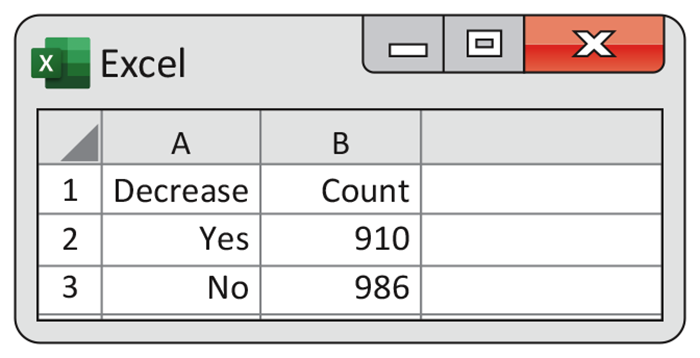
Figure 8.1 The robotics and jobs data in an Excel spreadsheet for the confidence interval, Example 8.3.
Figure 8.2 gives output from JMP and Minitab for these data. There are differences in the displays, but it is easy to find the 95% confidence interval. For JMP, the confidence interval is on the line with “Level” equal to Yes under the headings “Lower CI” and “Upper CI.” Minitab gives the output in the form of an interval under the heading “95% CI.” Notice that the confidence intervals are similar but not identical. Minitab notes that the Normal approximation is used. This is the large-sample method that we described. JMP notes that an alternative method, using score functions, is used.
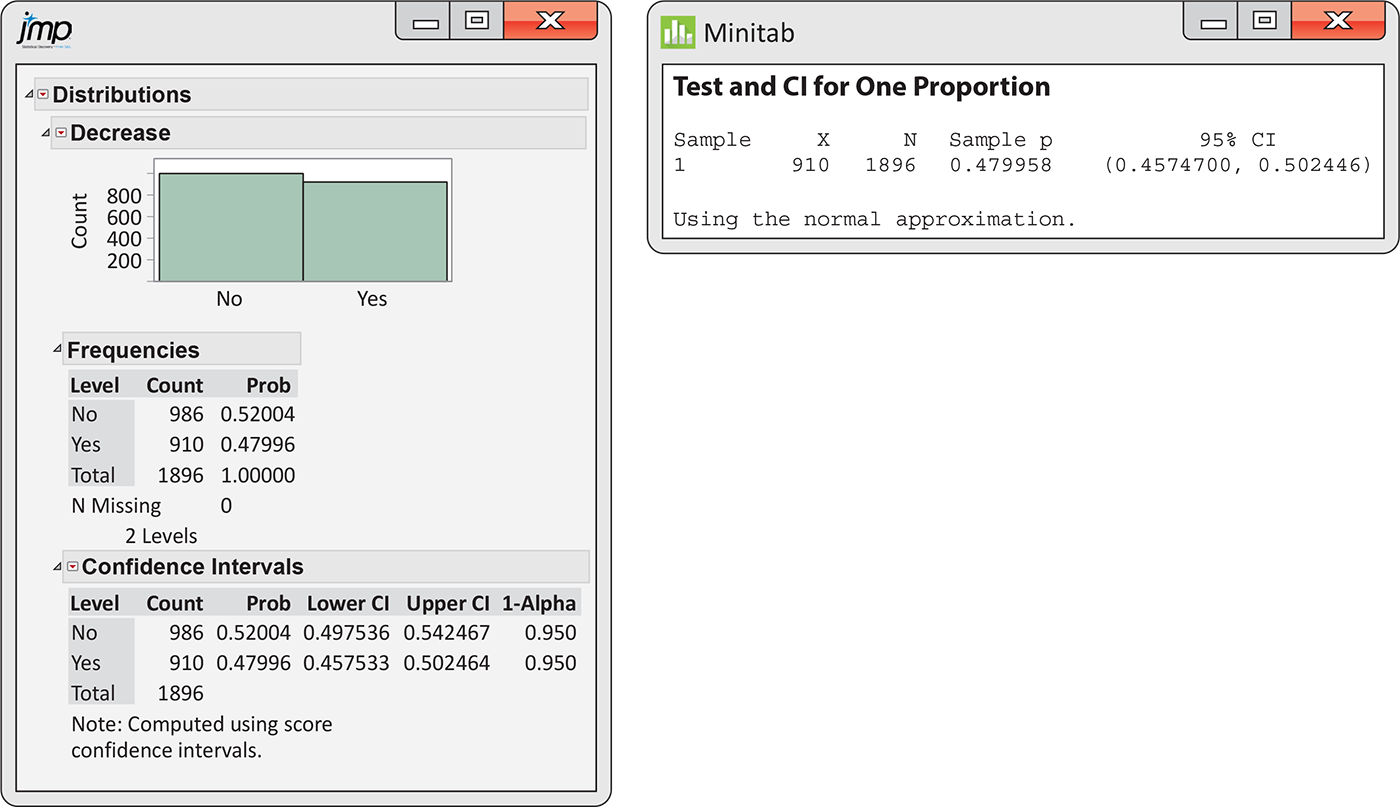
Figure 8.2 JMP and Minitab outputs for the robotics and jobs survey, Example 8.3.
As usual, the output reports more digits than are useful. When you use software, be sure to think about how many digits are meaningful for your purposes. Do not clutter your report with information that is not meaningful.
We recommend the large-sample confidence interval for 90%, 95%, and 99% confidence whenever the number of successes and the number of failures are both at least 10. For smaller sample sizes, we recommend exact methods that use the binomial distribution. These, as well as other alternative procedures, such as the score function, are available as the default or as options in many statistical software packages. We do not cover them here. There is also an intermediate case between large samples and very small samples where a slight modification of the large-sample approach works quite well. This method is called the “plus four” procedure and is described next.
Check-in
-
8.3 Users of Instagram. Refer to Check-in question 8.1 (page 451).
-
Find
-
Give the 95% confidence interval for p in the form of estimate plus or minus the margin of error.
-
Give the confidence interval as an interval of percents.
-
State your conclusion and interpret the meaning of the confidence interval in part (c).
-
-
8.4 Users of Snapchat. Refer to Check-in question 8.2 (page 451).
-
Find
-
Give the 95% confidence interval for p in the form of estimate plus or minus the margin of error.
-
Give the confidence interval as an interval of percents.
-
State your conclusion and interpret the meaning of the confidence interval in part (c).
-
Example 8.4 Plus four for the percent of equol producers.
Research has shown that there are many health benefits associated with a diet that contains soy foods. Substances in soy called isoflavones are known to be responsible for these benefits. When soy foods are consumed, some subjects produce a chemical called equol, and it is thought that production of equol is a key factor in the health benefits of a soy diet. Unfortunately, not all people are equol producers; there appear to be two distinct subpopulations: equol producers and equol nonproducers.
A nutrition researcher planning some bone health experiments would like to include some equol producers and some nonproducers among her subjects. A preliminary sample of 12 female subjects was measured, and 4 were found to be equol producers. We would like to estimate the proportion of equol producers in the population from which this researcher will draw her subjects.
The plus four estimate of the proportion of equol producers is
For a 95% confidence interval, we use
Table D
to find
and then the margin of error
So the confidence interval is
We estimate with 95% confidence that between 14% and 61% of women from this population are equol producers. Note that the interval is very wide because the sample size is very small. Compare this result with the large-sample confidence interval.
If the true proportion of equol users is near 14%, the lower limit of this interval, there may not be a sufficient number of equol producers in the study if subjects are tested only after they are enrolled in the experiment. It may be necessary to have a screening phase to determine whether or not a potential subject is an equol producer. The study could then be designed to have the same number of equol producers and nonproducers.
Significance test for a single proportion
![]()
Recall that the sample proportion
If the expected numbers of successes and failures are not both at least 10, or if the population is less than 20 times as large as the sample, other procedures should be used. One such approach is to use the binomial distribution, as we did with the sign test. Here is a large-sample matched-pairs example.
Example 8.5 Comparing two sunblock lotions.
![]()
Your company produces a sunblock lotion designed to protect the skin
from both UVA and UVB exposure to the sun. You hire a company to
compare your product with the product sold by your major competitor.
The testing company exposes skin on the backs of a sample of 20
people to UVA and UVB rays and measures the protection provided by
each product. For 13 of the subjects, your product provided better
protection, while for the other 7 subjects, your competitor’s
product provided better protection. Do you have evidence to support
a commercial advertisement claiming that your product provides
superior UVA and UVB protection? For the data we have
The expected numbers of successes (your product provides better
protection) and failures (your competitor’s product provides better
protection) are
The test statistic is
From
Table A, we find
We conclude that the sunblock testing data do not provide evidence
to reject the hypothesis of no difference between your product and
your competitor’s product
Note that we have used the two-sided alternative for this example. In settings like this, we must start with the view that either product could be better if we want to prove a claim of superiority. Thinking or hoping that your product is superior cannot be used to justify a one-sided test.
Although these calculations are not particularly difficult to do using a calculator, we prefer to use software. Here are some details.
Example 8.6 Sunblock significance tests using software.
![]()
JMP and Minitab outputs for the analysis in
Example 8.5 appear in
Figure 8.3. JMP uses a slightly different way of reporting the results. Two
ways of performing the significance test are labeled in the column
“Test.” The one that corresponds to the procedure that we have
described is on the second line, labeled “Pearson.” The
P-value under the heading “
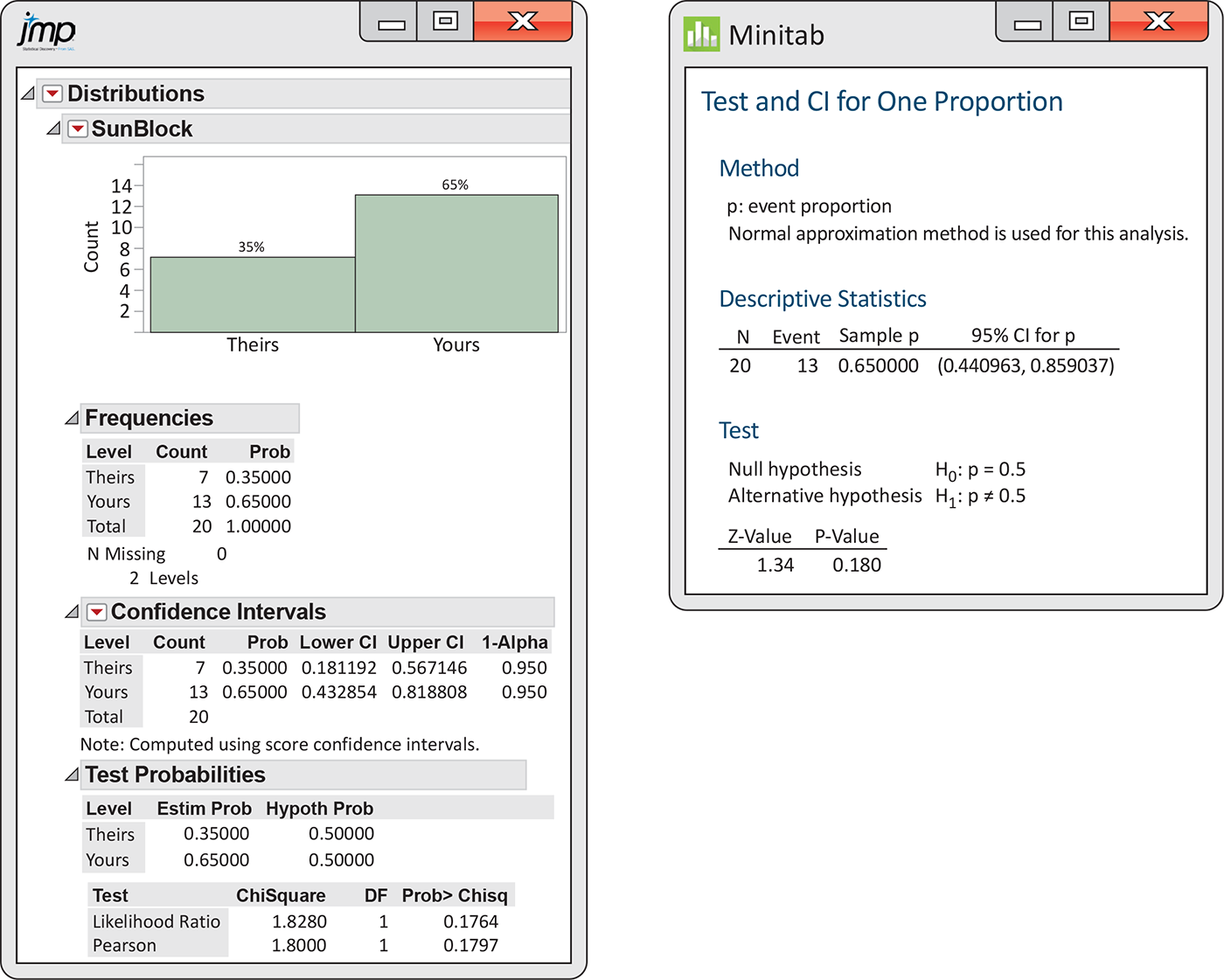
Figure 8.3 JMP and Minitab outputs for comparing sunblock lotions, Example 8.6.
Check-in
-
8.5 Draw a picture. Draw a picture of a standard Normal curve and shade the tail areas to illustrate the calculation of the P-value for Example 8.5.
-
8.6 What does the confidence interval tell us? Inspect the outputs in Figure 8.3. Report the confidence interval for the percent of people who would get better sun protection from your product than from your competitor’s. Be sure to convert from proportions to percents and to round appropriately. Interpret the confidence interval and compare this way of analyzing data with the significance test.
-
8.7 The effect of X. In Example 8.5 (page 457), suppose that your product provided better UVA and UVB protection for 16 of the 20 subjects. Perform the significance test and summarize the results.
-
8.8 The effect of n. In Example 8.5 (page 457), consider what would have happened if you had paid for three times as many subjects to be tested. Assume that the results would be similar to those in Example 8.5, that is, 65% of the subjects had better UVA and UVB protection with your product. Perform the significance test and summarize the results.
In Example 8.5, we treated an outcome as a success whenever your product provided better sun protection. Would we get the same results if we defined success as an outcome where your competitor’s product was superior? You will find in answering the next Check-in question that the answer is yes.
Check-in
-
8.9 Redefining success. In Example 8.5 (page 457), we performed a significance test to compare your product with your competitor’s. Success was defined as the outcome where your product provided better protection. Now, take the viewpoint of your competitor where success is defined to be the outcome where your competitor’s product provides better protection. In other words, n remains the same, but X is now 7.
-
Perform the two-sided significance test and report the results. How do these compare with what we found in Example 8.5?
-
Find the 95% confidence interval for this setting and compare it with the interval calculated when success is defined as the outcome where your product provides better protection.
-
![]() We do not often use significance tests for a single proportion
because it is uncommon to have a situation where there is a precise
We do not often use significance tests for a single proportion
because it is uncommon to have a situation where there is a precise
Data from past large samples can sometimes provide a
Choosing a sample size for a confidence interval
![]()
In Chapter 6, we showed how to choose the sample size n to obtain a confidence interval with specified margin of error m for a mean. Because we are using a Normal approximation for inference about a population proportion, sample size selection proceeds in much the same way.
Recall that the margin of error for the large-sample confidence interval for a population proportion is
Choosing a confidence level C fixes the critical value
z*. But the margin of error also depends on the data through
the value of
- Use the sample estimate from a pilot study or from similar studies done earlier.
-
Use
Once we have chosen p* and the margin of error m that we want, we can find the n we need to achieve this margin of error. Here is the result.
The value of n obtained by this method is not particularly
sensitive to the choice of p* when p* is fairly close to
0.5. However, if the value of p is likely to be smaller than
about 0.3 or larger than about 0.7, use of
Example 8.7 Planning a survey of students.
A large university is interested in assessing student satisfaction with the overall campus environment. The plan is to distribute a questionnaire to an SRS of students, but before proceeding, the university wants to determine how many students to sample. The questionnaire asks about a student’s degree of satisfaction with various student services, each measured on a five-point scale. The university is interested in the proportion p of students who are satisfied (that is, who choose either “satisfied” or “very satisfied,” the two highest levels on the five-point scale).
The university wants to estimate p with 95% confidence and
a margin of error less than or equal to 3%, or 0.03. For planning
purposes, it is willing to use
Round up to get
Similarly, for a 2.5% margin of error, we have (after rounding up)
and for a 2% margin of error,
News reports frequently describe the results of surveys with sample sizes between 1000 and 1500 and a margin of error of about 3%. These surveys generally use sampling procedures more complicated than simple random sampling, so the calculation of confidence intervals is more involved than what we have studied in this section. The calculations in Example 8.7 show in principle how such surveys are planned.
Example 8.8 Assessing interest in Pilates classes.

The Division of Recreational Sports (Rec Sports) at a major university is responsible for offering comprehensive recreational programs, services, and facilities to the students. Rec Sports is continually examining its programs to determine how well it is meeting the needs of the students. Rec Sports is considering adding some new programs and would like to know how much interest there is in a new exercise program based on the Pilates method.6 It will take a survey of undergraduate students. In the past, Rec Sports emailed short surveys to all undergraduate students. The response rate obtained in this way was about 5%. This time it will send emails to a simple random sample of the students and will follow up with additional emails and eventually a phone call to get a higher response rate. Because of limited staff and the work involved with the follow-up, it would like to use a sample size of about 200 responses. It assumes that the new procedures will improve the response rate to 90%, so it will contact 225 students in the hope that these will provide at least 200 valid responses. One of the questions it will ask is, “Have you ever heard about the Pilates method of exercise?”
The primary purpose of the survey is to estimate various sample
proportions for undergraduate students. Will the proposed sample size
of
Example 8.9 Margins of error.
In the Rec Sports survey, the margin of error of a 95% confidence
interval for any value of
The results for various values of
|
|
m |
|
m |
|---|---|---|---|
| 0.05 | 0.030 | 0.60 | 0.068 |
| 0.10 | 0.042 | 0.70 | 0.064 |
| 0.20 | 0.056 | 0.80 | 0.056 |
| 0.30 | 0.064 | 0.90 | 0.042 |
| 0.40 | 0.068 | 0.95 | 0.030 |
| 0.50 | 0.070 |
Rec Sports judged these margins of error to be acceptable, and it contacted 225 students, hoping to achieve a sample size of 200 for its survey.
The table in
Example 8.9 illustrates
two points. First, the margins of error for
![]() Again, it is important to emphasize that these calculations
consider only the effects of sampling variability that are
quantified in the margin of error.
Other sources of error, such as nonresponse and possible
misinterpretation of questions, are not included in the table of
margins of error for
Example 8.9. Rec Sports
is trying to minimize these kinds of errors. It performed a pilot
study using a small group of current users of its facilities to check
the wording of the questions, and for the final survey it devised a
careful plan to follow up with the students who did not respond to the
initial email.
Again, it is important to emphasize that these calculations
consider only the effects of sampling variability that are
quantified in the margin of error.
Other sources of error, such as nonresponse and possible
misinterpretation of questions, are not included in the table of
margins of error for
Example 8.9. Rec Sports
is trying to minimize these kinds of errors. It performed a pilot
study using a small group of current users of its facilities to check
the wording of the questions, and for the final survey it devised a
careful plan to follow up with the students who did not respond to the
initial email.
Check-in
-
8.10 Confidence level and sample size. Refer to Example 8.7 (page 460). Suppose that the university was interested in a 95% confidence interval with margin of error 0.02. Would the required sample size be smaller or larger than 1068 students? Verify your answer by performing the calculation.
-
8.11 Make a plot. Use the values for
Choosing a sample size for a significance test
In Chapter 6, we introduced the idea of power for a significance test. In Chapter 7, we discussed the relationship between sample size and power and described the use of software to calculate power for both one- and two-sample t tests. Those ideas also apply to the significance test for a proportion that we studied in this section. Thus, we can concentrate on the input and output and let software do the messy calculations.
To find the required sample size, we need to specify
-
The significance level
- Power (probability of rejecting the null hypothesis when it is false); usually we choose 80% (0.80) for power.
-
The value of
-
The alternative hypothesis, two-sided
- A value of p for the alternative hypothesis.
Example 8.10 Sample size for comparing two sunblock lotions.
In Example 8.5 (page 457), we performed the significance test for comparing two sunblock
lotions in a setting where each subject used the two lotions, and
the product that provided better protection was recorded. Although
your product performed better 13 times in 20 trials, the value
What sample size n should we choose if we want to have an 80%
chance of rejecting
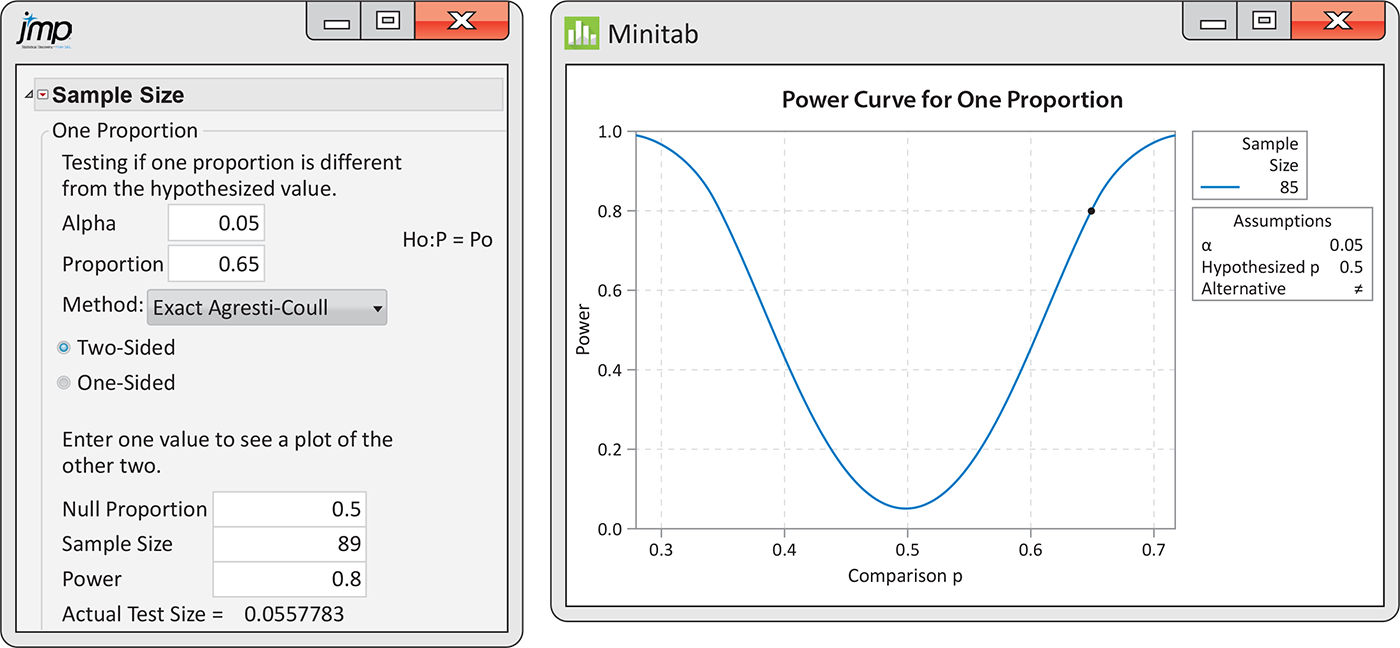
Figure 8.4 JMP and Minitab outputs for sample size needed to compare sunblock lotions, Example 8.10.
Note that Minitab provides a graph as a function of the value of the proportion for the alternative hypothesis. Similar plots can be produced by JMP. In some situations like those in Chapter 7, you might want to specify the sample size n and have software compute the power. This option is available in JMP, Minitab, and other software.
Check-in
-
8.12 Compute the sample size for a different alternative. Refer to Example 8.10. Use software to find the sample size needed for a two-sided test of the null hypothesis that
-
8.13 Compute the power for a given sample size. Consider the setting in Example 8.10. You have a budget that will allow you to test 50 subjects. Use software to find the power of the test for this value of n.
Section 8.1 Summary
-
Inference about a population proportion p from an SRS of size n is based on the sample proportion
-
For large samples, the level C margin of error of
where the critical value z* is the value for the standard Normal density curve with area C between
-
The level C large-sample confidence interval is
We recommend using this interval for 90%, 95%, and 99% confidence whenever the number of successes and the number of failures are both at least 10. When sample sizes are smaller, alternative procedures such as the plus four estimate of the population proportion are recommended.
-
Tests of
with P-values calculated from the N(0, 1) distribution. Use this procedure when the expected number of successes,
-
The sample size required to obtain a confidence interval of approximate margin of error m for a proportion is found from
where p* is a guessed value for the proportion and z* is the standard Normal critical value for the desired level of confidence. To ensure that the margin of error of the interval is less than or equal to m no matter what
-
Software can be used to determine the sample sizes for significance tests. Inputs include the significance level, the desired power, the null hypothesized value of p, and the alternative value of p.
Section 8.1 EXERCISES
-
8.1 Do you use a smart watch or fitness tracker? A Pew Internet poll asked 4272 U.S. adults about their use of smart watches and fitness trackers. A summary of the results reported that 897 adults regularly wear a smart watch or fitness tracker.7
Identify the sample size and the count.
Calculate the sample proportion.
-
Explain the relationship between the population proportion and the sample proportion.
-
8.2 What do you know about science? A Pew Internet poll tested 4464 U.S. adults about their knowledge of science. One of the questions asked how far a car will travel in 45 minutes if it travels at a constant speed of 40 miles per hour. Possible answers presented were 25 miles, 30 miles, 35 miles, and 45 miles. The correct answer was given by 2544 adults.8
Identify the sample size and the count.
Calculate the sample proportion.
-
Explain the relationship between the population proportion and the sample proportion.
-
8.3 Analysis of the smart watch or fitness tracker data. Refer to Exercise 8.1.
-
Report the sample proportion, the standard error of the sample proportion, and the margin of error for 95% confidence.
-
Are the guidelines for when to use the large-sample confidence interval for a population proportion satisfied in this setting? Explain your answer.
-
Find the 95% large-sample confidence interval for the population proportion.
-
Write a short statement explaining the meaning of your confidence interval.
-
-
8.4 Analysis of the science knowledge data. Refer to Exercise 8.2.
-
Report the sample proportion, the standard error of the sample proportion, and the margin of error for 95% confidence.
-
Are the guidelines for when to use the large-sample confidence interval for a population proportion satisfied in this setting? Explain your answer.
-
Find the 95% large-sample confidence interval for the population proportion.
-
Write a short statement explaining the meaning of your confidence interval.
-
-
8.5 Would you recommend the service to a friend? An automobile dealership asks all its customers who used its service department in a given two-week period if they would recommend the service to a friend. A total of 200 customers used the service during the two-week period, and 180 said that they would recommend the service to a friend.
Identify the sample size and the count.
Calculate the sample proportion.
-
Explain the relationship between the population proportion and the sample proportion.
-
8.6 Analysis of the service recommendation data. Refer to the previous exercise.
-
Report the sample proportion, the standard error of the sample proportion, and the margin of error for 95% confidence.
-
Are the guidelines for when to use the large-sample confidence interval for a population proportion satisfied in this setting? Explain your answer.
-
Find the 95% large-sample confidence interval for the population proportion.
-
Write a short statement explaining the meaning of you confidence interval.
-
-
8.7 Whole grain versus regular grain? A study of young children was designed to increase their intake of whole-grain, rather than regular-grain, snacks. At the end of the study, the 82 children who participated in the study were presented with a choice between a regular-grain snack and a whole-grain alternative. The whole-grain alternative was chosen by 49 children. You want to examine the possibility that the children are equally likely to choose each type of snack.
-
Formulate the null and alternative hypotheses for this setting.
-
Are the guidelines for using the large-sample significance test satisfied for testing this null hypothesis? Explain your answer.
-
Perform the significance test and summarize your results in a short paragraph.
-
-
8.8 What’s wrong? For each of the following statements, explain what is wrong and why.
-
You can use a significance test to evaluate the hypothesis
-
The large-sample significance test for a population proportion is based on a t statistic.
-
An approximate 95% confidence interval for an unknown proportion p is
-
-
8.9 Find the sample size. You are planning a survey similar to the one about the use of smart watches and fitness trackers described in Exercise 8.1. You will report your results with a large-sample 95% confidence interval. How large a sample do you need to be sure that the margin of error will not be greater than 0.02? Show your work, including what you used to choose a value for p*.
-
8.10 Draw some pictures. Consider the binomial setting with
-
The sample proportion
-
Draw a sketch of this Normal distribution. Mark the location of the mean.
-
Find a value p* for which the probability is 95% that
-
-
8.11 Country food and Inuits. Country food includes seals, caribou, whales, ducks, fish, and berries and is an important part of the diet of the aboriginal people called Inuits who inhabit Inuit Nunangat, the northern region of what is now called Canada. A survey of Inuits in Inuit Nunangat reported that 3274 out of 5000 respondents said that at least half of the meat and fish that they eat is country food.9 Find the sample proportion and a 95% confidence interval for the population proportion of Inuits whose meat and fish consumption consists of at least half country food.
-
8.12 Soft drink consumption in New Zealand. A survey commissioned by the Southern Cross Healthcare Group reported that 16% of New Zealanders consume five or more servings of soft drinks per week. The data were obtained through an online survey of 2006 randomly selected New Zealanders over 15 years of age.10
-
What number of survey respondents reported that they consume five or more servings of soft drinks per week? You will need to round your answer. Why?
-
Find a 95% confidence interval for the proportion of New Zealanders who report that they consume five or more servings of soft drinks per week.
-
Convert the estimate and your confidence interval to percents.
Discuss reasons the estimate might be biased.
-
-
8.13 Violent video games. A survey of 1050 parents who have a child under the age of 18 living at home asked about their opinions regarding violent video games. A report describing the results of the survey stated that 89% of parents say that violence in today’s video games is a problem.11
-
What number of survey respondents reported that they thought that violence in today’s video games is a problem? You will need to round your answer. Why?
-
Find a 95% confidence interval for the proportion of parents who think that violence in today’s video games is a problem.
-
Convert the estimate and your confidence interval to percents.
Discuss reasons the estimate might be biased.
-
-
8.14 Bullying. Refer to the previous exercise. The survey also reported that 93% of the parents surveyed said that bullying contributes to violence in the United States. Answer the questions in the previous exercise for this item on the survey.
-
8.15
-
Find the values of the sample proportion
-
Repeat part (a), assuming a sample size of
-
Make a sketch illustrating what you have found in parts (a) and (b). What does your sketch show about the effect of the sample size in this setting?
-
-
8.16 Students doing community service. In a sample of 159,949 first-year college students, the National Survey of Student Engagement reported that 39% participated in community service or volunteer work.12
Find the margin of error for 99% confidence.
-
Here are some facts from the report that summarizes the survey. The students were from 617 four-year colleges and universities. The response rate was 36%. Institutions paid a participation fee of between $1800 and $7800, based on the size of their undergraduate enrollment. Discuss these facts as possible sources of error in this study. How do you think these errors would compare with the margin of error that you calculated in part (a)?
-
8.17 Plans to study abroad. The survey described in the previous exercise also asked about items related to academics. In response to one of these questions, 42% of first-year students reported that they planned to study abroad.
-
Based on the information available, how many students planned to study abroad?
-
Give a 99% confidence interval for the population proportion of first-year college students who planned to study abroad.
-
-
8.18 Student credit cards. In a survey of 1430 undergraduate students, 1087 reported that they had one or more credit cards.13 Give a 95% confidence interval for the proportion of all college students who had at least one credit card.
-
8.19 How many credit cards? The summary of the survey described in the previous exercise reported that 43% of undergraduates had four or more credit cards. Give a 95% confidence interval for the proportion of all college students who had four or more credit cards.
-
8.20 How would the confidence interval change? Refer to the previous exercise.
-
Would a 90% confidence interval be wider or narrower than the one that you found in the previous exercise? Verify your answer by computing the interval.
-
Would a 97% confidence interval be wider or narrower than the one that you found in that exercise? Verify your results by computing the interval.
-
-
8.21 Do students report Internet sources? The National Survey of Student Engagement found that 87% of students report that their peers at least “sometimes” copy information from the Internet in their papers without reporting the source.14 Assume that the sample size is 430,000.
Find the margin of error for 99% confidence.
-
Here are some items from the report that summarizes the survey. More than 430,000 students from 730 four-year colleges and universities participated. The average response rate was 43% and ranged from 15% to 89%. Institutions pay a participation fee of between $3000 and $7500 based on the size of their undergraduate enrollment. Discuss these facts as possible sources of error in this study. How do you think these errors would compare with the error that you calculated in part (a)?
-
8.22 Can we use the z test? In each of the following cases, state whether or not the Normal approximation to the binomial should be used for a significance test on the population proportion p. Explain your answers.
-
-
 8.23 Long sermons.
The National Congregations Study collected data in a one-hour
interview with a key informant—that is, a minister, priest,
rabbi, or other staff person or leader.15
One question concerned the length of the typical sermon. For
this question, 390 out of 1191 congregations reported that the
typical sermon lasted more than 30 minutes.
8.23 Long sermons.
The National Congregations Study collected data in a one-hour
interview with a key informant—that is, a minister, priest,
rabbi, or other staff person or leader.15
One question concerned the length of the typical sermon. For
this question, 390 out of 1191 congregations reported that the
typical sermon lasted more than 30 minutes.
-
Use the large-sample inference procedures to estimate the true proportion for this question with a 95% confidence interval.
-
The respondents to this question were not asked to use a stopwatch to record the lengths of a random sample of sermons at their congregations. They responded based on their impressions of the sermons. Do you think that ministers, priests, rabbis, or other staff persons or leaders might perceive sermon lengths differently from the people listening to the sermons? Discuss how your ideas would influence your interpretation of the results of this study.
-
-
8.24 Instant versus fresh-brewed coffee. A matched pairs experiment compares the taste of instant with fresh-brewed coffee. Each subject tastes two unmarked cups of coffee, one of each type, in random order, and states which they prefer. Of the 50 subjects who participate in the study, 32 preferred the fresh-brewed coffee.
-
Test the claim that a majority of people preferred the taste of fresh-brewed coffee. Report the large-sample z statistic and its P-value.
-
Draw a sketch of a standard Normal curve and mark the location of your z statistic. Shade the appropriate area that corresponds to the P-value.
-
Is your result significant at the 5% level? What is your practical conclusion?
-
-
8.25 Tossing a coin 10,000 times! The South African mathematician John Kerrich, while a prisoner of war during World War II, tossed a coin 10,000 times and obtained 5067 heads.
-
Is this significant evidence at the 5% level that the probability that Kerrich’s coin comes up heads is not 0.5? Use a sketch of the standard Normal distribution to illustrate the P-value.
-
Use a 95% confidence interval to find the range of probabilities of heads that would not be rejected at the 5% level.
-
-
8.26 Is there interest in a new product? One of your employees has suggested that your company develop a new product. You decide to take a random sample of your customers and ask whether or not there is interest in the new product. The response is on a 1 to 5 scale with 1 indicating “definitely would not purchase”; 2, “probably would not purchase”; 3, “not sure”; 4, “probably would purchase”; and 5, “definitely would purchase.” For an initial analysis, you will record the responses 1, 2, and 3 as No and 4 and 5 as Yes. What sample size would you use if you wanted the 95% margin of error to be 0.20 or less?
-
8.27 More information is needed. Refer to the previous exercise. Suppose that after reviewing the results of the previous survey, you proceeded with preliminary development of the product. Now you are at the stage where you need to decide whether or not to make a major investment to produce and market it. You will use another random sample of your customers, but now you want the margin of error to be smaller. What sample size would you use if you wanted the 95% margin of error to be 0.01 or less?
-
8.28 Sample size needed for an evaluation. You are planning an evaluation of a semester-long alcohol awareness campaign at your college. Previous evaluations indicate that about 25% of the students surveyed will respond Yes to the question “Did the campaign alter your behavior toward alcohol consumption?” How large a sample of students should you take if you want the margin of error for 95% confidence to be about 0.06?
-
8.29 Find more sample sizes.
The evaluation in the previous exercise will also have questions
that have not been asked before, so you do not have previous
information about the possible value of p. Repeat the
preceding calculation for the following values of p*:
0.1, 0.2, 0.3, 0.4, 0.5, 0.6, 0.7, 0.8, and 0.9. Summarize the
results in a table and graphically. What sample size will you
use?
-
8.30 Are the customers dissatisfied? An automobile manufacturer would like to know what proportion of its customers are dissatisfied with the service received from their local dealer. The customer relations department will survey a random sample of customers and compute a 95% confidence interval for the proportion who are dissatisfied. From past studies, it believes that this proportion will be about 0.30. Find the sample size needed if the margin of error of the confidence interval is to be no more than 0.04.
-
8.31 Sample size for coffee. Refer to Exercise 8.24, where we analyzed data from a matched pairs study that compared preferences for instant versus fresh-brewed coffee. Suppose that you want to design a similar study. The null hypothesis is that instant and fresh-brewed are equally likely to be preferred, and the alternative is two-sided. You will use
-
8.32 Sample size for tossing a coin. Refer to Exercise 8.25, where we analyzed the 10,000 coin tosses made by John Kerrich. Suppose that you want to design a study that would test the hypothesis that a coin is fair versus the alternative that the probability of a head is 0.52. Using a two-sided test with
-
8.33 What’s wrong? For each of the following statements, explain what is wrong and why.
-
The margin of error for a confidence interval used for an opinion poll takes into account the fact that people who did not answer the poll questions would have given the same responses as those who did answer the questions.
-
If the P-value for a significance test is 0.05, we can conclude that the null hypothesis has a 5% chance of being true.
-
A student project used a confidence interval to describe the results in a final report. The confidence level was 115%.
-