12.2 Comparing the Means
The ANOVA F test gives a general answer to a general question: Are the differences among observed group means statistically significant? Unfortunately, a small P-value simply tells us that the group means are not all the same. It does not tell us specifically which means differ from each other. Plotting and inspecting the means give us some indication of where the differences lie, but we would like to supplement inspection with formal inference. This section presents two approaches to the task of comparing group means. It concludes with discussion on the power of the one-way ANOVA F test.
Contrasts
In the ideal situation, specific questions regarding comparisons among the means are posed before the data are collected. We can answer specific questions of this kind and attach a level of confidence to the answers we give. We now explore these ideas through a Facebook study.
Example 12.18 How do users spend their time on Facebook?
![]()

An online study was designed to compare the amount of time a Facebook user devotes to reading positive, negative, and neutral Facebook profiles. Each participant was randomly assigned to one of five Facebook profile groups:
- Positive female
- Positive male
- Negative female
- Negative male
- Gender neutral with neutral content
Each participant was provided an email link to a survey on Survey Monkey. As part of the survey, the participant was directed to view the assigned Facebook profile page and then answer some questions. The amount of time (in minutes) the participant spent viewing the profile prior to answering the questions was recorded as the response.10
We should always begin our analysis with a check of the data. Time-to-event data (here, the time until the participant begins to answer the survey questions) is often skewed to the right. Preliminary analysis of the residuals (Figure 12.11) confirms this.
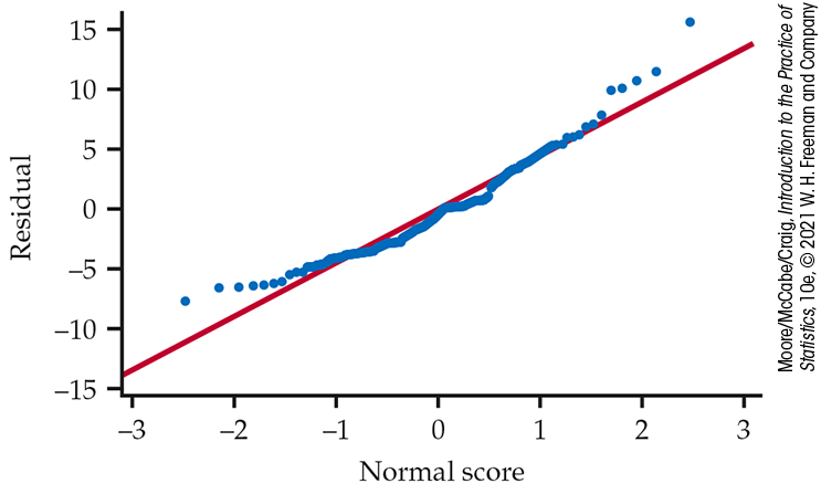
Figure 12.11 Normal quantile plot of residuals from one-way ANOVA fit to time-to-event data, Example 12.18.
As a result, we consider the square root of time for analysis.
These results are summarized in
Figures 12.12
and 12.13. The residuals
appear approximately Normal (Figure 12.12), and our rule for examining standard deviations indicates that we
can assume equal population standard deviations
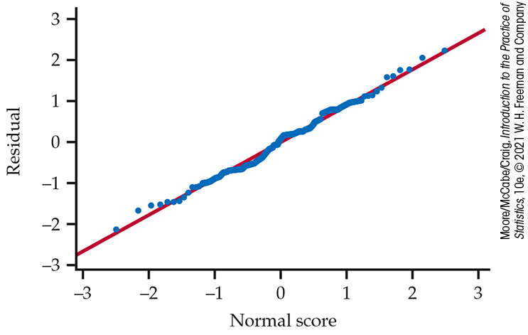
Figure 12.12 Normal quantile plot of residuals from one-way ANOVA fit to transformed time-to-event data, Example 12.18.
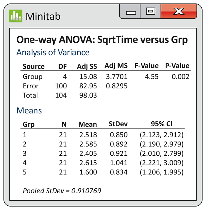
Figure 12.13 Minitab output giving the one-way ANOVA table for the Facebook profile study after the square root transformation, Example 12.18.
![]()
The F test is significant with a P-value of 0.002.
Because the P-value is very small, there is strong evidence
against
Rejecting the null hypothesis
and concluding that the five population means are not the same does not tell us all we’d like to know. We would really like our analysis to provide us with more specific information. For example, the alternative hypothesis is true if
or if
or if
![]() When you reject the ANOVA null hypothesis, additional analyses are
required to clarify the nature of the differences between the
means.
When you reject the ANOVA null hypothesis, additional analyses are
required to clarify the nature of the differences between the
means.
For this study, the researcher predicted that participants would spend more time viewing the negative Facebook pages compared to the positive or neutral pages because the negative pages would stand out more and thus garner more attention. (This is called cognitive salience.) How do we translate these predictions into testable hypotheses?
Example 12.19 A comparison of interest.
The researcher hypothesizes that participants exposed to a negative Facebook profile would spend more time viewing the page than would participants who are exposed to a positive Facebook profile. Because two groups are exposed to negative profiles and two are exposed to positive profiles, we can consider the following null hypothesis:
versus the two-sided alternative
We could argue that the one-sided alternative
is appropriate for this problem, provided that other evidence suggests this direction and is not just what the researcher wants to see.
In the preceding example, we used
Example 12.20 Another comparison of interest.
This comparison tests whether there is a difference in time between groups exposed to a negative page and the group exposed to the neutral page. Here are the null and alternative hypotheses:
Each of
and for the second comparison
In each case, the value of the contrast is 0 when
![]() Note that we have chosen to define the contrasts so that they will
be positive when the alternative of interest (what we expect) is
true. Whenever possible, this is a good idea because it makes results
easier to read.
Note that we have chosen to define the contrasts so that they will
be positive when the alternative of interest (what we expect) is
true. Whenever possible, this is a good idea because it makes results
easier to read.
A contrast expresses an effect in the population as a combination of population means. To estimate the contrast, form the corresponding sample contrast by using sample means in place of population means. Under the ANOVA assumptions, a sample contrast is a linear combination of independent Normal variables and, therefore, has a Normal distribution (page 49). We can obtain the standard error of a contrast by using the rules for variances. Inference is based on t statistics. Here are the details.
Because each
Example 12.21 The contrast coefficients.
For the contrasts in Examples 12.19 and 12.20, the coefficients are
and
where the subscripts 1, 2, 3, 4, and 5 correspond to the profiles
listed in
Example 12.17, respectively. In each case, the sum of the
We now look at inference for each of these contrasts in turn.
Example 12.22 Testing the first contrast of interest.
The sample contrast that estimates
with standard error
The t statistic for testing
Because
We use the same method for the second contrast.
Example 12.23 Testing the second contrast of interest.
The sample contrast that estimates
with standard error
The t statistic for assessing the significance of this contrast is
The P-value for the two-sided alternative is 0.0003. If we
use
Table D, we conclude that
The size of the difference can be described with a confidence interval.
Example 12.24 Confidence interval for the second contrast.
To find the 95% confidence interval for
The interval is (0.43, 1.39). Unfortunately, this interval is
difficult to interpret because the units are
JMP output for the two contrasts is given in Figure 12.14. The results agree with the calculations that we performed in Examples 12.22 and 12.23 except for minor differences due to roundoff error in our calculations. Note that the output does not give the confidence interval that we calculated in Example 12.24. This is easily computed, however, from the contrast estimate and standard error provided in the output.
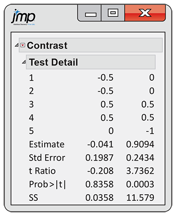
Figure 12.14 JMP output giving the contrast analysis for the Facebook profile study.
Some statistical software packages report the test statistics associated with contrasts as F statistics rather than t statistics. These F statistics are the squares of the t statistics described previously. As with much other statistical software output, P-values for significance tests are reported for the two-sided alternative.
![]() If the software you are using gives P-values for the two-sided
alternative, and you are using the appropriate one-sided
alternative, divide the reported P-value by 2.
In our example, we argued that a one-sided alternative may be
appropriate for the first contrast. The software reported the
P-value as 0.836, so we can conclude
If the software you are using gives P-values for the two-sided
alternative, and you are using the appropriate one-sided
alternative, divide the reported P-value by 2.
In our example, we argued that a one-sided alternative may be
appropriate for the first contrast. The software reported the
P-value as 0.836, so we can conclude
Questions about population means are expressed as hypotheses about contrasts. A contrast should express a specific question that we have in mind when designing the study. Because the ANOVA F test answers a very general question, it is less powerful than tests for contrasts designed to answer specific questions.
![]() When contrasts are formulated before seeing the data, inference
about contrasts is valid whether or not the ANOVA
When contrasts are formulated before seeing the data, inference
about contrasts is valid whether or not the ANOVA
Check-in
-
12.13 Defining a contrast. Refer to Example 12.18 (page 620). Suppose the researcher was also interested in comparing the viewing time between male and female profile pages. Specify the coefficients for this contrast.
-
12.14 Defining different coefficients. Refer to Example 12.23 (page 628). Suppose we had selected the coefficients
Multiple comparisons
![]()
In many studies, specific questions cannot be formulated in advance of
the analysis. If
Example 12.25 Comparing each pair of groups.
Let’s return once more to the Facebook study with five groups (page 624). We can make 10 comparisons between pairs of means. We can write a t statistic for each of these pairs. For example, the statistic
compares Profiles 1 and 2. The subscripts on t specify which groups are compared.
The t statistics for two other pairs are
and
These 10 t statistics are very similar to the pooled two-sample
t statistic for comparing two population means. The difference
is that we now have more than two populations, so each statistic uses
the pooled estimator
Because we do not have any specific ordering of the means in mind as an alternative to equality, we must use a two-sided approach to the problem of deciding which pairs of means are significantly different.
One obvious choice for
![]() The LSD method has some undesirable properties, particularly if the
number of means being compared is large. Suppose, for example, that there are
The LSD method has some undesirable properties, particularly if the
number of means being compared is large. Suppose, for example, that there are
Because LSD fixes the probability of a false rejection for each
single pair of means being compared, it does not control the
overall probability of some false rejection among all pairs.
Other choices of
We will discuss only one of these, called the Bonferroni method. Use
of this method with
Example 12.26 Applying the Bonferroni method.
We apply the Bonferroni method to the data from the Facebook study
using an overall
Of course, we prefer to use software for the calculations.
Example 12.27 Interpreting software output.
The output generated by SPSS for comparisons using the Bonferroni method appears in Figure 12.15. Here, all 10 comparisons are reported. In fact, each comparison is given twice. The software uses an asterisk to indicate that the difference in a pair of means is statistically significant. These results agree with our conclusions for the three comparisons in Example 12.26.
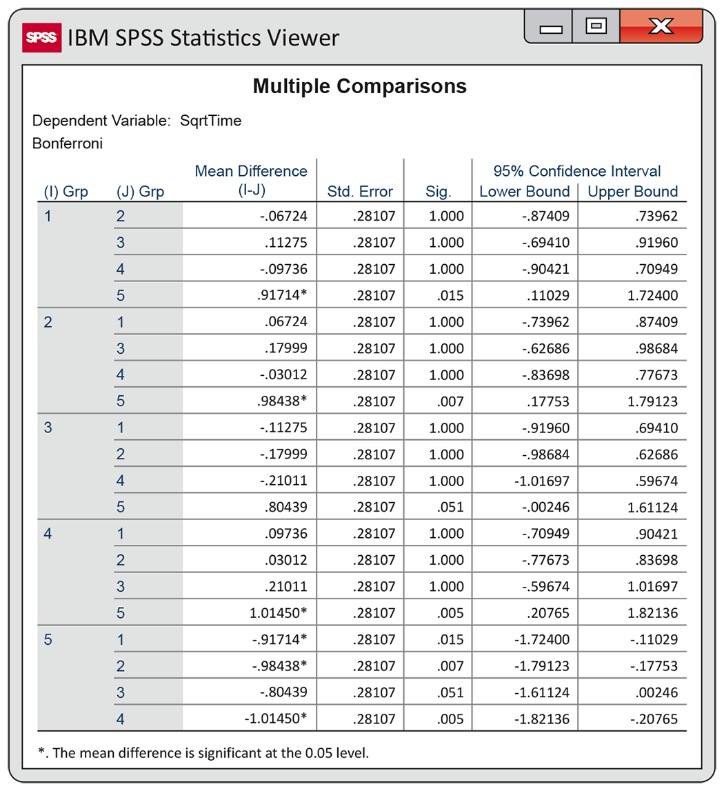
Figure 12.15 SPSS output giving the multiple-comparisons analysis for the Facebook profile study, Example 12.27.
SPSS does not provide the t statistic but rather a
Bonferroni-adjusted P-value for the comparisons under the
heading “Sig.” The Bonferroni-adjusted P-value is obtained by
multiplying the unadjusted P-value by the number of
comparisons. When this is greater than 1, the adjusted
P-value is reported as 1.000. In the “Sig.” column, there are
only three comparisons with a P-value smaller than the
overall
When there are a large number of groups, it is often difficult to concisely describe the numerous results of multiple comparisons. Instead, researchers often list the means and use letters to label the pairs that are not found to be statistically different.
Example 12.28 Displaying multiple-comparisons results.
The following table lists the groups of the Facebook study, with
their sample sizes, means, and standard deviations. The groups are
ordered by
| Profile | n |
|
s |
|---|---|---|---|
| 4. Negative male | 21 |
|
1.041 |
| 2. Positive male | 21 |
|
0.892 |
| 1. Positive female | 21 |
|
0.850 |
| 3. Negative female | 21 |
|
0.921 |
| 5. Neutral | 21 |
|
0.834 |
Here, the mean associated with Profile 5 is significantly different from the means for Profile 1, 2, and 4 because they do not have a common label. Profile 5 is not found to be significantly different from the mean for Profile 3 because they share the label “B.” To complicate things, the means for Profiles 1, 2, and 4 are also not found to be significantly different from the mean of Profile 3 as they share the label “A.”
The conclusions from this table in
Example 12.28 appear to
be illogical. If
This apparent contradiction points out the nature of the conclusions
of statistical tests of significance. In the multiple-comparison
setting, these tests ask, “Do we have adequate evidence to distinguish
two means?” In describing the results, we should talk about failing to
detect a difference or concluding that two groups are different. We
also must remember that
failing to find strong enough evidence that two means differ
doesn’t say that they are equal. Thus, it is not illogical to conclude that we have sufficient
evidence to distinguish
Simultaneous confidence intervals
One way to deal with the difficulties of interpretation is to give confidence intervals for the differences. The intervals remind us that the differences are not known exactly. We also want to give simultaneous confidence intervals—that is, intervals for all differences among the population means at once. Again, we must face the problem that there are many competing procedures—in this case, many methods of obtaining simultaneous intervals.
The confidence intervals generated by a particular choice of
Example 12.29 Interpreting software output (continued).
The SPSS output for the Bonferroni method given in
Figure 12.15 also includes
simultaneous 95% confidence intervals in the last two columns. We
can see, for example, that the Bonferroni interval for
Check-in
-
12.15 Why no additional analyses? Explain why it is unnecessary to further analyze the data using a multiple-comparisons method when
-
12.16 Growth of Douglas fir seedlings. An experiment was conducted to compare the growth of Douglas fir seedlings under three different levels of vegetation control (0%, 50%, and 100%). Sixteen seedlings were randomized to each level of control. The resulting sample means for stem volume were 58, 73, and 105 cubic centimeters
-
What are the coefficients for testing this contrast?
-
Perform the test and report the test statistic, degrees of freedom, and P-value. Do the data provide evidence to support this hypothesis?
-
Power of the one-way ANOVA F test
The power of a statistical test is a measure of the test’s ability to detect deviations from the null hypothesis. In Chapter 7, we described the use of power calculations to ensure adequate sample size for inference about means in one- and two-population studies. In this section, we extend these methods to any number of populations.
Because the one-way ANOVA F test is a generalization of the two-sample t test, it should not be surprising that the procedure for calculating power of the F test is quite similar. In both cases, the following four study specifications are needed to compute power:
-
Significance level
- Common population standard deviation
- Group sample sizes
-
Specific alternative
The difference comes in the specific calculations. Instead of using a
t and noncentral t distribution to compute the
probability of rejecting
The last three study specifications in the prior list determine the
appropriate noncentral F distribution. Most software assumes a
constant sample size n for the group sizes. For the
alternative, some software doesn’t request group means but rather the
smallest difference between means that is judged practically
important. Here is an example using two software packages that
approach specifying
Example 12.30 Power of a reading comprehension study.
Suppose that a study on reading comprehension for three different teaching methods has 10 students in each group. How likely is this study to detect differences in means? A previous study, using the same three teaching methods but performed in a different setting, found sample means of 40, 48, and 42, and the pooled standard deviation was 7. We’ll use these values to compute the power for this new study.
Figure 12.16
shows the power calculation output from JMP and Minitab. In both
cases, we use
For JMP, we enter the alternative group means and the total sample
size
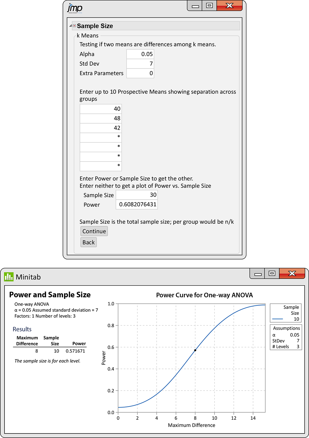
Figure 12.16 JMP and Minitab power calculation outputs, Example 12.30.
As in this case, the power is usually lower when only specifying an important difference between means. This is because the other population means are not specified, and so the software considers a worst-case scenario.
If the assumed values of the
Example 12.31 Changing the sample size.
To decide on an appropriate sample size for the experiment described in the previous example, we repeat the power calculation for different values of n, the number of subjects in each group. Here are the results:
| N | DFG | DFE | F* | Power |
|---|---|---|---|---|
| 30 | 2 | 27 | 3.35 | 0.61 |
| 36 | 2 | 33 | 3.28 | 0.70 |
| 45 | 2 | 42 | 3.22 | 0.81 |
| 57 | 2 | 54 | 3.17 | 0.90 |
| 99 | 2 | 96 | 3.09 | 0.99 |
When you have a level of power in mind, software will allow you to
directly solve for the necessary sample size rather than trying
different values for n, as we did in this example. Instead of
leaving the power blank, you’d enter the desired power as an input
(usually 80% or 90%) and leave the sample size blank. Try this out
using JMP for the setting of
Example 12.31 and verify
that the experimenters need
A study with 90% power means the experimenters have a 90% chance of
rejecting
There is, however, a cost associated with this increased power. The total sample size is almost doubled, which could mean a doubling of the cost of the study. To trade off cost with the risk of not detecting the difference in the means, researchers generally shoot for power in the 80% to 90% range. In most real-life situations, the additional cost of increasing the sample size so that the power is very close to 100% cannot be justified.
Check-in
-
12.17 Understanding power calculations. Refer to Example 12.30. Suppose that the researcher decided to use
-
12.18 Understanding power calculations (continued). If all the group means are equal (
Section 12.2 SUMMARY
-
The ANOVA F test does not say which group means differ. It is, therefore, usual to add comparisons among the means to one-way ANOVA.
-
Specific questions formulated before examination of the data can be expressed as contrasts. Tests and confidence intervals for contrasts provide answers to these questions.
-
If no specific questions are formulated before examination of the data and the null hypothesis of equality of population means is rejected, multiple-comparisons procedures are used to assess the statistical significance of the differences between pairs of means.
-
The least significant differences (LSD) method controls the probability of a false rejection for each comparison. The Bonferroni method controls the overall probability of some false rejections among all comparisons.
-
The power of the one-way ANOVA F test depends upon the significance level, the group sample sizes, the common population standard deviation, and the choice of alternative. Software can do the power calculations if these study-specific factors are provided.
Section 12.2 EXERCISES
-
12.20 Define a contrast. An ANOVA was run with six groups. Give the coefficients for the contrast that compares the average of the means of the first four groups with the mean of the last two groups.
-
12.21 Find the standard error. Refer to the previous exercise. Suppose that there are 10 observations in each group and that
-
12.22 Is the contrast significant? Refer to the previous exercise. Suppose that the average of the first four groups minus the average of the last two groups is 2.6. State an appropriate null hypothesis for this comparison and find the test statistic with its degrees of freedom. Can you draw a conclusion? Or do you need to know the alternative hypothesis?
-
12.23 Give the confidence interval. Refer to the previous exercise. Give a 95% confidence interval for the difference between the average of the means of the first four groups and the average mean of the last two groups.
-
12.24 Background music contrast. Refer to Example 12.3 (page 603). The researchers hypothesize that listening to any background music (with or without lyrics) will, on average, result in fewer completed math problems than working in silence. Test this hypothesis with a contrast. Make sure to specify the null and alternative hypotheses, the sample contrast, and its standard error. Also report the t statistic, along with its degrees of freedom and P-value.

-
12.25 College dining facilities. University and college food service operations have been trying to keep up with the growing expectations of consumers with regard to the overall campus dining experience. Because customer satisfaction has been shown to be associated with repeat patronage and new customers gained through word of mouth, a public university in the Midwest took a sample of patrons from its eating establishments and asked them about their overall dining satisfaction.11 The following table summarizes the results for three groups of patrons:
Category n s Student—meal plan 3.44 489 0.804 Faculty—meal plan 4.04 69 0.824 Student—no meal plan 3.47 212 0.657 -
Is it reasonable to use a pooled standard deviation for these data? Why or why not? If yes, compute it.
-
The ANOVA F statistic was reported as 17.66. Give the degrees of freedom and either an approximate (from a table) or an exact (from software) P-value. Sketch a picture that describes this calculation.
-
Prior to performing this survey, food service operations thought that satisfaction among faculty on the meal plan would be higher than satisfaction among students on the meal plan. Explain why a contrast should be used to examine this rather than a multiple-comparisons procedure.
-
Use the results in the table to test this contrast. Make sure to specify the null and alternative hypotheses, test statistic, and P-value.
-
Suppose food service operations had been interested in comparing faculty on the meal plan to students overall. Repeat part (d) using this question on interest.
-
-
12.26 Writing contrasts. You’ve been asked to help some administrators analyze survey data on textbook expenditures collected at a large public university. Let
-
Because first- and second-year students take lower-level courses, which often involve large introductory textbooks, the administrators want to compare the average textbook expenditures of the first-year and second-year students with those of the third- and fourth-year students. Write a contrast that expresses this comparison.
-
Write a contrast for comparing the mean of the first-year students with that of the second-year students.
-
Write a contrast for comparing the mean of the third-year students with that of the fourth-year students.
-
-
12.27 Writing contrasts (continued). Return to the eye study described in Example 12.16 (page 618). Let
-
Because a majority of the population in this study are Hispanic (eye color predominantly brown), we want to compare the average score of the brown eyes with the average of the other two eye colors. Write a contrast that expresses this comparison.
-
Write a contrast to compare the average score when the model is looking at the viewer versus the average score when the model is looking down.
-
-
12.28 Analyzing contrasts. Answer the following questions for the two contrasts that you defined in the previous exercise.

-
For each contrast, give
-
Find the values of the corresponding sample contrasts
-
Calculate the standard errors
-
Give the test statistics and approximate P-values for the two significance tests. What do you conclude?
-
Compute 95% confidence intervals for the two contrasts.
-
-
12.29 Two contrasts of interest for the stimulant study. Refer to Exercise 12.15 (page 623). There are two comparisons of interest to the experimenter. They are (1) placebo versus the average of the two low-dose treatments and (2) the difference between High A and Low A versus the difference between High B and Low B.
-
Express each contrast in terms of the means
-
Give estimates with standard errors for each of the contrasts.
-
Perform the significance tests for the contrasts. Summarize the results of your tests.
-
-
12.30 The Bonferroni method. For each of the following settings, state the α level to be used for each test.
-
There are 21 pairs of means
-
There are 36 pairs of means
-
There are
-
-
12.31 Use of a multiple-comparisons procedure. A friend performed a one-way ANOVA at the
-
12.32 Multitasking with technology in the classroom. Laptops and other digital technologies with wireless access to the Internet are becoming more and more common in the classroom. While numerous studies have shown that these technologies can be used effectively as part of teaching, there is concern that these technologies can also distract learners if used for off-task behaviors.
In one study that looked at the effects of off-task multitasking with digital technologies in the classroom, a total of 145 undergraduates were randomly assigned to one of seven conditions.12 Each condition involved performing a task simultaneously during lecture. The study consisted of three 20-minute lectures, each followed by a 15-item quiz. The following table summarizes the conditions and quiz results (mean proportion correct):
Condition n Lecture 1 Lecture 2 Lecture 3 Texting 21 0.57 0.75 0.56 Emailing 20 0.52 0.69 0.50 Using Facebook 20 0.50 0.68 0.43 MSN messaging 21 0.48 0.71 0.42 Natural use control 21 0.50 0.78 0.58 Word-processing control 21 0.55 0.75 0.57 Paper-and-pencil control 21 0.60 0.74 0.53 -
For this analysis, let’s consider the average of the three quizzes as the response. Compute this mean for each condition.
-
The analysis of these average scores results in
-
Using the means from part (a) and the Bonferroni method, determine which pairs of means differ significantly at the 0.05 significance level. (Hint: There are 21 pairwise comparisons, so the critical t-value is 3.095. Also, it is best to order the means from smallest to largest to help with pairwise comparisons.)
-
Summarize your results from parts (b) and (c) in a short report.
-
-
12.33 Contrasts for multitasking. Refer to the previous exercise. Let
-
The researchers hypothesized that the average score for the off-task behaviors would be lower than that for the paper-and-pencil control condition. Write a contrast that expresses this comparison.
-
For this contrast, give
-
Calculate the test statistic and approximate P-value for the significance test. What do you conclude?
-
-
12.34 Power calculations for planning a study. You are planning a new eye gaze study for a different university than that studied in Example 12.16 (page 618). From Figure 12.9 (page 618), the pooled standard error is 1.68. To be a little conservative, use
-
Pick several values for n (the number of students that you will select for each group) and calculate the power of the ANOVA F test for each of your choices.
-
Plot the power versus the sample size. Describe the general shape of the plot.
-
What choice of n would you choose for your study? Give reasons for your answer.
-
-
12.35 Power for a different alternative. Refer to the previous exercise. Suppose we increase