14.1 The Logistic Regression Model in Chapter 14 Logistic Regression

14.1 The Logistic Regression Model

Binomial distributions and odds

In Chapter 5 we studied binomial distributions, and in Chapter 8 we learned how to do statistical inference for the proportion p of successes in the binomial setting. We start with a brief review of some of these ideas that we will need in this chapter.

Example 14.1 Do you eat breakfast regularly?

A random sample of 300 students from your college was asked if they regularly eat breakfast. Of these students, 180 responded that they eat breakfast regularly.

Using the notation of Chapter 5, p is the proportion of students in the population of students in your college who eat breakfast regularly. Assuming that the population is much larger than the SRS of size n, the number of students who would respond that they eat breakfast regularly has the binomial distribution with parameters n and p. For this survey, the sample size is n=300, and the count who responded that they eat breakfast regularly is X=180. The sample proportion is

p^=180300=0.6

Based on this SRS, we estimate that 60% of the students at your college eat breakfast regularly.

Logistic regressions work with odds rather than proportions. The odds are simply the ratio of the proportions for the two possible outcomes. If p^ is the proportion for one outcome, then 1−p^ is the proportion for the second outcome, and

odds=p^1−p^

A similar formula for the population odds is obtained by substituting p for p^ in this expression.

Example 14.2 Odds of eating breakfast regularly.

For the breakfast eating data, the proportion of students who responded that they eat breakfast regularly is p^=0.6, so the proportion of students who answered that they did not eat breakfast regularly is

1−p^=1−0.6=0.4

Therefore, the odds of eating breakfast regularly are

odds=p^1−p^=0.60.4=1.5

When people speak about odds, they often express odds using integers or fractions. We calculated the odds as 1.5, but we could have also expressed it as 3/2. Thus, we could say that the odds are 3 to 2 that a student eats breakfast regularly. We could also say that for every three students who say they eat breakfast regularly, there are two students who do not. We could also describe the odds of not eating breakfast regularly as 2 to 3.

Check-in

14.1 Odds of drawing an ace. If you deal one card from a standard deck, the probability that the card is an ace is 4/52=1/13.
1. Find the odds of drawing an ace.
2. Find the odds of drawing a card that is not an ace.
14.2 Given the odds, find the probability. If you know the odds, you can find the probability by solving the odds equation for the probability. So, p^=odds/(odds+1). If the odds of an outcome are 3.5 (or 7 to 2), what is the probability of the outcome?

Odds for two groups

In Example 8.11 (page 469) we compared the return rates of lost wallets with money and without money. Using the methods of Chapter 8, we compared the proportions of returned wallets with a confidence interval (page 470) and with a significance test (page 475).

Example 14.3 Comparing the returns of wallets with money and without money.

Data set for lost.

Figure 14.1 contains output from JMP for this comparison. The sample proportion of returned wallets with money is given as 58%, and the sample proportion for wallets with no money is 37%. These entries are the row percents in the two-way table. The difference is 0.211, and the 95% confidence interval is (0.130715, 0.286504). We can summarize this result by saying, “The percent of returned wallets with money is 21% higher than the percent of wallets returned without money. 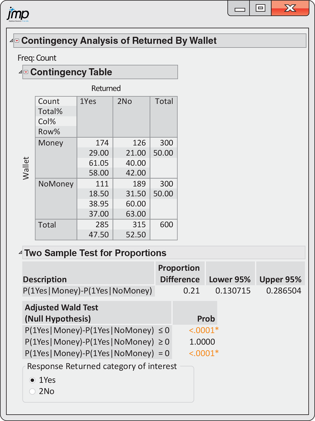This difference is statistically significant (P<0.0001) and the 95% confidence interval is 13% to 29%.”

A JMP output for a contingency analysis. — Figure 14.1 JMP output for the comparison of the proportions of returned wallets with money and with no money, Example 14.3.

The output shows an expanded dropdown list menu, contingency analysis returned by wallet. It lists frequency, count. Another expanded menu, contingency table, shows a table where rows represent wallet and columns represent returned. A key identifies the output in each cell of the table. Each cell lists four values which represent the following in order, count, total percentage, column percentage, row percentage. The data is as follows. Wallet, money. Returned, yes, 174, 29.00, 61.05, 58.00. Retuned, no, 126, 21.00, 40.00, 42.00. Total count wallet money, 300. Total percentage wallet money, 50.00. Wallet, no money. Returned, yes. 111, 18.50, 38.95, 37.00. Returned, no. 189, 31.50, 60.00, 63.00. Total count wallet no money, 300. Total percentage wallet no money, 50.00. Total count returned yes, 285. Total percentage returned yes, 47.50. Total count returned no, 315. Total percentage returned no, 52.50. Another expanded menu, two sample test for proportions, shows two tables with the following data. First table. Description, P 1 yes, money minus P 1 yes no money. Proportion difference, 0.21. Lower 95 percent, 0.130715. Upper 95 percent, 0.286504. Second table, adjusted Wald test. Null hypothesis, P 1 yes money minus P 1 yes no money less than or equal to 0. Probability, less that 0.0001 asterisk. Null hypothesis, P 1 yes money minus P 1 yes no money greater than or equal to 0. Probability, 1.0000. Null hypothesis, P 1 yes money minus P 1 yes no money = 0. Probability, less than 0.0001 asterisk. Radio buttons are shown for the option response returned category of interest, 1 yes or 2 n0. 1 yes is selected.

We could also describe the difference in percents using odds.

Example 14.4 Odds for lost wallets being returned.

Data set for lost.

For wallets with money,

odds=p^1−p^=0.581−0.58=1.381

Similarly, for wallets without money we have

odds=p^1−p^=0.371−0.37=0.5873

Check-in

14.3 Physical education requirements. In Exercise 8.41 (page 482) you examined the proportion in higher education institutions that had a physical education requirement. For the 225 private institutions, 60 had a requirement. For the 129 public universities, 101 had a requirement. Find the odds of having a physical education requirement for the private institutions. Do the same for the public institutions.
14.4 Find the odds. Refer to the previous Check-in question. Find the odds of not having a physical education requirement for the private institutions. Do the same for the public institutions.

Model for logistic regression

In simple linear regression, we modeled the mean μ of the response variable y as a linear function of the explanatory variable: μ=β0+β1x. When y is just 1 or 0 (success or failure), the mean is the probability p of a success. Logistic regression models the mean p in terms of an explanatory variable x. We might try to relate p and x as in simple linear regression: p=β0+β1x. Unfortunately, this is not a good model. Whenever β1≠0, extreme values of x will give values of β0+β1x that fall outside the range of possible values of p, 0≤p≤1.

The logistic regression solution to this difficulty is to transform the odds p/(1−p) using the natural logarithm. We use the term log odds or logit for this transformation.

Example 14.5 Log odds for lost wallets.

Data set for lost.

For wallets with money,

log(odds)=log(1.381)=0.3228

and for wallets without money,

log(odds)=log(0.5873)=−0.5322

For the lost wallets data, the explanatory variable is money, a categorical variable. To use a categorical explanatory variable in a logistic regression, we usually use a numerical code. We can do this with an indicator variable. For our problem, we will use an indicator of whether the wallet contains money:

x={ 1 if the wallet contains money0 if the wallet does not contain money

We model the log odds as a linear function of the explanatory variable:

log(p1−p)=β0+β1x

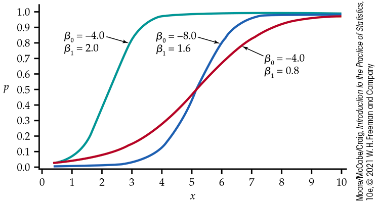
Note that the right-hand side of this equation is the same as the function that we used for the mean of y in the simple linear regression model (page 519). Figure 14.2 graphs the relationship between p and x for some different values of β0 and β1. For logistic regression, we use natural logarithms.

A graph of P versus x with three plots. — Figure 14.2 Plot of p versus x for different logistic regression models.

The graph plots P on the vertical axis, ranging from 0.0 to 1.0 in increments of 0.1, versus x on the vertical axis, ranging from 0 to 10 in increments of 1. Three S shaped curves are plotted. A plot for Beta sub 0 = negative 4.0 and Beta sub 1 = 2.0 rises with increasing steepness from (0.5, 0.02) and through (2, 0.3) to an inflection point at (2, 0.5), then rises with decreasing steepness to (5, 0.95), then extends roughly horizontally. A plot for Beta sub 0 = negative 8.0, Beta sub 1 = 1.6 rises with increasing steepness from (0.5, 0.01) and through (4, 0.1) to an inflection point at (5, 0.5), then rises with decreasing steepness through (6.5, 0.9) to (7.5, 0.95), then extends roughly horizontally. A plot for Beta sub 0 = negative 4.0, Beta sub 1 = 0.8 rises with increasing steepness from (0.5, 0.02) and through (4, 0.3) to an inflection point at (5, 0.5), then rises with decreasing steepness through (7.5, 0.8) and (10, 0.95). All values estimated.

Check-in

14.5 Find the log odds. Refer to Check-in question 14.3. Find the log odds for having a physical education requirement for private institutions. Do the same for public institutions.
14.6 Find the log odds. Refer to Check-in question 14.4. Find the log odds for not having a physical education requirement for private institutions. Do the same for public institutions.

In Chapter 10 we studied inference for simple linear regression, a model with one explanatory variable x. In Chapter 11, we extended the model to the case where there can be several explanatory variables, x1, x2, … xk, where k is the number of explanatory variables. The same ideas apply to logistic regression. Here is the general model.

As we did with least-squares regression, we use the term simple logistic regression for models with a single explanatory variable and multiple logistic regression for models with more than one explanatory variable. In the latter case, each regression coefficient expresses the effect of the variable when all other explanatory variables are held constant.

Example 14.6 Model for lost wallets.

Data set for lost.

For our lost wallets example, there are n=600 wallets in the sample. The explanatory variable is whether the wallet contains money, which we have coded using an indicator variable with values x=1 for wallets with money and x=0 for wallets without money. The model says that the probability p that a wallet is returned can depend upon the whether the wallet has money in it (x=1 or x=0). So there are two possible values for p—say, pwith money and pwithout money.

The logistic regression model specifies the relationship between p and x. Because there are only two values for x, we write both equations. For wallets with money,

log(pwith money1−pwith money)=β0+β1

and for wallets without money,

log(pwithout money1−pwithout money)=β0

Note that there is a β1 term in the equation for wallets with money because x=1, but it is missing in the equation for wallets without money because x=0.

Logistic regression with an indicator explanatory variable is a very special case. It is important because many multiple logistic regression analyses focus on one or more such variables as the primary explanatory variables of interest. For now, we use this special case to understand a little more about the model.

Fitting and interpreting the logistic regression model

In general, the calculations needed to find the estimates b0 and b1 for the parameters β0 and β1 are complex and require the use of software. When the explanatory variable has only two possible values, however, we can easily find the estimates by replacing the log odds with their estimates from the data.

Example 14.7 Log odds and b1 for lost wallets.

Data set for lost.

In Example 14.5, we found the log odds for wallets with money,

log(p^with money1−p^with money)=0.3228

and for wallets without money,

log(p^without money1−p^without money)=−0.5322

The logistic regression model for money is

log(pwith money1−pwith money)=β0+β1

and for no money, it is

log(pwithout money1−pwithout money)=β0

To find the estimates b0 and b1, we match the with and without money model equations with the corresponding data equations. Thus, we see that the estimate of the intercept b0 is simply the log odds for the without money wallets:

b0=−0.5322

and the estimate of b1 is the difference between the log odds for with money and the log odds for without money:

b1=0.3228−(−0.5322)=0.8550

The fitted logistic regression model is

log(odds)=−0.5322+0.8550x

The coefficient b1 in this logistic regression model is the difference between the log odds for no money and the log odds for money. Many people are uncomfortable thinking in the log odds scale, so interpretation of the results in terms of the regression coefficient b1 is difficult. Usually, we apply a transformation to help us. With a little algebra, it can be shown that

eb1=oddswith moneyoddswithout money

The transformation eb1 undoes the logarithm and transforms the b1 into an odds ratio.

Example 14.8 Odds ratio for lost wallets.

Data set for lost.

For the lost wallet data, the odds ratio is the odds that a wallet with money (x=1) is returned divided by the odds that a wallet without money (x=0) is returned. In Example 14.4, we calculated oddswith money=1.381 and oddswithout money=0.5873. So, for the lost wallets example, we see

oddswith moneyoddswithout money=1.3810.5873=2.351=eb1

We can multiply the odds for without money by the odds ratio to obtain the odds for with money:

oddswith money=2.351×oddswithout money

In this case, we would say that the odds for with money are about two and a third times the odds for without money.

Notice that we have chosen the coding for the indicator variable so that the regression coefficient b1 is positive. This will give an odds ratio that is greater than 1. Had we coded without money as 1 and with money as 0, the sign of the regression coefficient b1 would be reversed and the odds ratio would be e−0.8550=0.4253. The odds for without money are about 40% of the odds for with money.

Logistic regression with an explanatory variable having two values is a very important special case. Here is an example where the explanatory variable is quantitative.

Example 14.9 Is a movie going to be profitable?

Data set icon for movies.

The MOVIES data file includes both the movie’s budget and the total U.S. revenue for 76 movies. For this example, we will classify each movie as profitable (y=1) if U.S. revenue is larger than the budget and not profitable (y=0) otherwise. Profit is our response variable. The data file contains several explanatory variables, but we will focus here on the natural logarithm of the opening-weekend revenue (x=LOpening). Figure 14.3 is a scatterplot of the data with a scatterplot smoother. The probability that a movie is profitable increases with the log opening-weekend revenue. Let’s fit the logistic regression model

log(p1−p)=β0+β1x

where p is the probability that the movie is profitable and x is the log opening-weekend revenue. The model for estimated log odds fitted by software is

log(odds)=b0+b1x=−2.56+1.125x

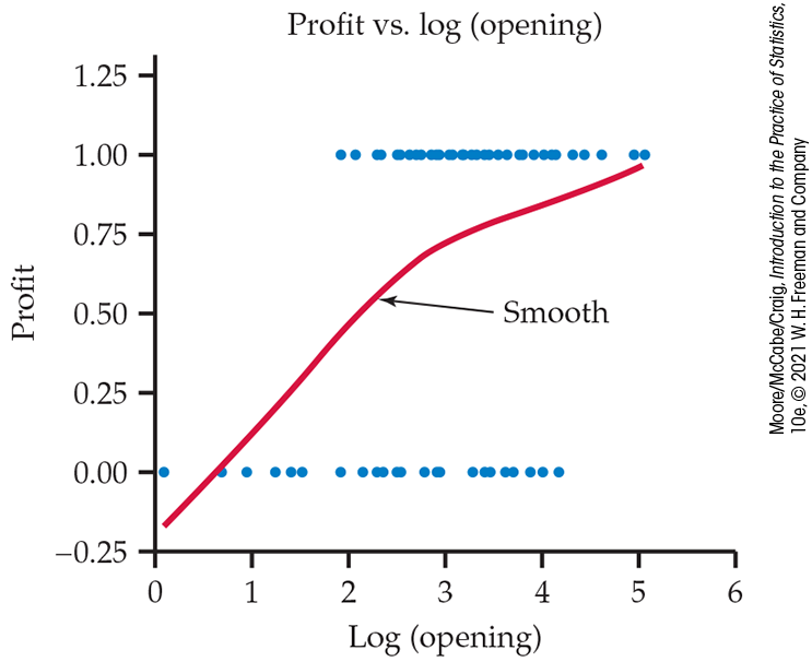
The odds ratio is eb1=3.08. This means that if log opening-weekend revenue (x) increases by one unit (roughly $2.71 million), the odds that the movie will be profitable increase by a factor of 3.08.

A scatterplot of profit versus log of opening. — Figure 14.3 Scatterplot of profit (Y=1, N=0) versus the log of opening weekend revenue with a smooth function, Example 14.9.

Check-in

14.7 Find the logistic regression equation and the odds ratio. Refer to Check-in questions 14.3 and 14.5. Find the logistic regression equation and the odds ratio.
14.8 Find the logistic regression equation and the odds ratio. Refer to Check-in questions 14.4 and 14.6. Find the logistic regression equation and the odds ratio.

Section 14.1 SUMMARY

If p^ is the sample proportion, then the odds are p^/(1−p^), the ratio of the proportion of times the event happens to the proportion of times the event does not happen.
The logistic regression model relates the log odds or logit to the explanatory variables:

log(p1−p)=β0+β1x1+β2x2+…+βkxk

Here p is a binomial proportion of successes, and x1, x2, … xk are the k explanatory variables.
The parameters of the logistic regression model are β0, β1, … βk.
For the explanatory variable xi, the odds ratio is eβi. It is the ratio of the odds for the data corresponding to a change of one unit in the explanatory variable.

Now that you have completed this section, you will be able to:

Find the odds of an outcome from its probability. Review Example 14.2 (page 14-3) and try Exercise 14.1.
Describe the statistical model for logistic regression. Review Example 14.6 (page 14-6) and try Exercise 14.5.
Find and interpret an odds ratios. Review Example 14.8 (page 14-8) and try Exercise 14.5.

Section 14.1 EXERCISES

14.1 What purchases will be made? A poll of 1200 adults aged 18 or older asked about purchases they intended to make for the upcoming holiday season. A total of 543 adults listed gift card as a planned purchase.
1. What proportion of adults plan to purchase a gift card as a present?
2. What are the odds that an adult will purchase a gift card as a present?
3. What proportion of adults do not plan to purchase a gift card as a present?
4. What are the odds that an adult will not buy a gift card as a present?
5. How are your answers to parts (b) and (d) related?
14.2 How did you use your cell phone? One question in a Pew Internet Poll on cell phone use asked whether, during the past 30 days, the person had used their phone while in a store to call a friend or family member for advice about a purchase they were considering. The poll surveyed 1003 adults living in the United States. Of these, 462 responded that they had used their cell phones for this purpose.²
1. What proportion of those surveyed reported that they used their cell phones while in a store within the past 30 days to call a friend or family member for advice about a purchase they were considering?
2. Find the odds for using the phone for the purpose in part (a).
14.3 Find some odds. For each of the following probabilities, find the odds: 0.1, 0.2, 0.3, 0.4, 0.5, 0.6, 0.7, 0.8, 0.9. Make a plot of the odds versus the probabilities and describe the relationship.
14.4 A logistic regression for teeth and military service. Exercise 8.40 (page 481) describes data on the numbers of U.S. recruits who were rejected for service in a war against Spain because they did not have enough teeth. The exercise compared the rejection rate for recruits who were under the age of 20 with the rate for those who were 40 or over. To run a logistic regression for this setting, we define an indicator explanatory variable (x=Age) with values 0 for age under 20 and 1 for age 40 or over. Figure 14.4 gives output from Minitab for this analysis.
1. How many recruits were examined? How many were rejected, and how many were not rejected?
2. Write the fitted logistic regression model.
3. Demonstrate how to obtain the odds ratio from the table of coefficients.
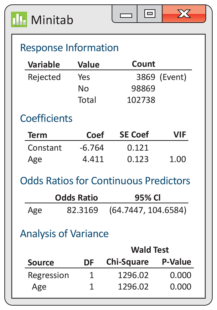
Figure 14.4 Minitab logistic regression output for predicting recruit rejection using age in two categories, for Exercises 14.4, 14.13, 14.15, and 14.22.

The output shows four tables of data as follows. First table, response information. Variable, rejected. Value, yes. Count, 3869, event. Value, no. Count, 98869. Value, total. Count, 102738. Second table, coefficients. Term, constant. Coefficient, negative 6.764. S E coefficient, 0.121. V I F, blank. Term, age. Coefficient, 4.411. S E coefficient, 0.123. V I F, 1.00. Third table, odds ratios for continuous predictors. Level, age. Odds ratio, 82.3169. 95 percent C I, (64.7447, 104.6584). Fourth table, analysis of variance. Source, regression. D F, 1. Wald test, chi square, 1296.02. Wald test P-vale, 0.000. Source, age. D F, 1. Wald test chi square, 1296.02. Wald test P-value, 0.000.
14.5 A logistic model for cell phones. Refer to Exercise 14.2. Suppose that you want to investigate differences in cell phone use among customers of different ages. You create an indicator explanatory variable x that has the value 1 if the customer is 25 years of age or less and 0 if the customer over 25 years of age.
1. Describe the statistical model for logistic regression in this setting.
2. Explain the relationship between the regression coefficients and the odds ratios for the two groups of customers defined by x.
14.6 High blood pressure and cardiovascular disease. There is much evidence that high blood pressure is associated with increased risk of death from cardiovascular disease. A major study of this association examined 3351 men with high blood pressure and 2654 men with low blood pressure. During the period of the study, 20 men in the low-blood-pressure group and 57 in the high-blood-pressure group died from cardiovascular disease.
1. Find the proportion of men who died from cardiovascular disease in the high-blood-pressure group. Then calculate the odds.
2. Do the same for the low-blood-pressure group.
3. Now calculate the odds ratio with the odds for the high-blood-pressure group in the numerator. Describe the result in words.
14.7 What’s wrong? For each of the following, explain what is wrong and why.
1. The intercept β0 is equal to the odds of an event when x=0.
2. The log odds of an event are 1 minus the probability of the event.
3. If b1=3 in a logistic regression analysis with one explanatory variable, we estimate that the probability of an event is multiplied by 3 when the value of the explanatory variable increases by one unit.
14.8 Will a movie be profitable? In Example 14.9 (page 14-9), we described a model to predict whether a movie is profitable based on log opening-weekend revenue (x=LOpening). What are the predicted odds of a movie being profitable if the opening-weekend revenue is
1. $20 million dollars (x=3.10)?
2. $40 million dollars (x=3.26)?
3. $60 million dollars (x=4.42)?
14.9 Convert the odds to probabilities. Refer to the previous exercise. For each opening-weekend revenue, compute the estimated probability that the movie is profitable.

14.10 Salt intake and cardiovascular disease. In Example 9.13 (page 501), the relative risk of developing cardiovascular disease (CVD) for people with low- and high-salt diets was estimated. Let’s reanalyze these data using the methods in this chapter. Here are the data:

Developed CVD	Salt in diet
Developed CVD	Low	High	Total
Yes	88	112	200
No	1081	1134	2215
Total	1169	1246	2415

For each salt level, find the probability of developing CVD.
Convert each of the probabilities that you found in part (a) to odds.
Find the log of each of the odds that you found in part (b).

14.11 Salt in the diet and CVD. Refer to the previous exercise. Use x=1 for the high-salt diet and x=0 for the low-salt diet.
1. Find the estimates b0 and b1.
2. Give the fitted logistic regression model.
3. What is the odds ratio for a high-salt versus low-salt diet?
4. When the probability of an event is very small, the odds ratio and relative risk are similar. Compare this odds ratio with the relative risk estimate in Example 9.13. Are they close? Explain your answer.

NAEP 14.12 Internet use in Canada. A recent study used data from the Canadian Internet Use Survey (CIUS) to explore the relationship between certain A variables and Internet use by individuals in Canada.³ The response variable refers to the use of the Internet from any location within the last 12 months. Explanatory variables included Age (years), Income (thousands of dollars), Location (1=urban, 0=other), Sex (1=male, 0=female), Education (1=at least some postsecondary education, 0=other), Language (1=English, 0=French), and Children (1=at least one child in household, 0=no Children). The following table summarizes the results:

Explanatory variable	b
Age	−0.063
Income	0.013
Location	0.367
Sex	−0.222
Education	1.080
Language	0.285
Children	0.049
Intercept	2.010

All but Children were significant at the 0.05 level.

Interpret the sign of each of the coefficients (except the intercept) in terms of the probability that the individual uses the Internet.
Compute the odds ratio for each of the variables in the table.
What are the odds that a French-speaking, 23-year-old male, living alone in Montreal and making $50,000 a year his second year after college is using the Internet?
Convert the odds in part (c) to a probability.