11.1 Inference for Multiple Regression
Population multiple regression equation
The simple linear regression model assumes that the mean of the response variable y depends on the explanatory variable x according to a linear equation
For any fixed value of x, the response y varies Normally
about this mean and has a standard deviation
In the multiple regression setting, the response variable
y depends on p explanatory variables, which we will
denote by
Similar to simple linear regression, this expression is the population regression equation, and the observed values y vary about their means given by this equation.
Just as we did in simple linear regression, we can also think of this
model in terms of subpopulations of responses. Here, each
subpopulation corresponds to a particular set of values for
all the explanatory variables
Example 11.1 Predicting early success in college.
Our case study is based on data collected on science majors at a large university.1 The goal of the study was to develop a model to predict success in the early university years. Success was measured using the cumulative grade point average (GPA) after three semesters. The explanatory variables were achievement scores available at the time of enrollment in the university. These included their average high school grades in mathematics (HSM), science (HSS), and English (HSE).
We will use high school grades to predict the response variable GPA.
There are
The population multiple regression equation for the mean GPAs is
For the straight-C subpopulation of students, the equation gives the mean as
Data for multiple regression
The data for a simple linear regression problem consist of
n pairs of a response variable y and an explanatory
variable x. Because there are several explanatory variables in
multiple regression, the notation needed to describe the data is more
elaborate. Each observation, or case, consists of a value for the
response variable and for each of the explanatory variables. Call
Here, n is the number of cases, and p is the number of explanatory variables. Data are often entered into computer regression programs in this format. Each row is a case, and each column corresponds to a different variable.
Example 11.2 The data for predicting early success in college.
![]()
The data for
Example 11.1, with several additional explanatory variables, appear in this
format in the GPA data file.
Figure 11.1
shows the first six rows entered into an Excel spreadsheet. Grade
point average (GPA) is the response variable, followed by
The six achievement scores are all quantitative explanatory variables. Sex is an indicator variable using the numerical values 0 and 1 to represent male and female, respectively.
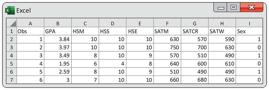
Figure 11.1 Format of the data set for predicting success in college, Example 11.2.
Indicator variables are used frequently in multiple regression to represent the levels or groups of categorical explanatory variable. See Exercises 11.16 through 11.18 (pages 574–575) for more discussion of their use in a multiple regression model.
Check-in
-
11.1 Describing a multiple regression. To minimize the negative impact of math anxiety on achievement in a research design course, a group of investigators implemented a series of feedback sessions, in which the teacher went over the small-group assignments and discussed the most frequently committed errors.2 At the end of the course, data from 166 students were obtained. The investigators studied how students’ final exam scores were explained by math course anxiety, math test anxiety, numerical task anxiety, enjoyment, self-confidence, motivation, and perceived usefulness of the feedback sessions.
What is the response variable?
-
What are the cases, and what is n, the number of cases?
-
What is p, the number of explanatory variables?
What are the explanatory variables?
Multiple linear regression model
Similar to simple linear regression, we combine the population regression equation and the assumptions about how the observed y vary about their means to construct the multiple linear regression model. The subpopulation means describe the FIT part of our conceptual model
The RESIDUAL part represents the variation of observed y about their means.
We will use the same notation for the residual that we used in the
simple linear regression model. The symbol
The assumption that the subpopulation means are related to the
regression coefficients
implies that we can estimate all subpopulation means from the
estimates of the
We also need to be cautious when interpreting each of the regression
coefficients in a multiple regression. First, the
![]() Second, the description provided by the regression coefficient of
each x variable is similar to that provided by the slope in
simple linear regression but only in a specific situation—namely,
when all other x variables are held constant. We need this extra condition because with multiple
x variables, it is quite possible that a unit change in one
x variable may be associated with changes in other
x variables. If that occurs, then the overall change in the
mean of y is not described by just a single regression
coefficient.
Second, the description provided by the regression coefficient of
each x variable is similar to that provided by the slope in
simple linear regression but only in a specific situation—namely,
when all other x variables are held constant. We need this extra condition because with multiple
x variables, it is quite possible that a unit change in one
x variable may be associated with changes in other
x variables. If that occurs, then the overall change in the
mean of y is not described by just a single regression
coefficient.
Check-in
-
11.2 Understanding the fitted regression line. The fitted regression equation for a multiple regression is
-
If
-
For the answer to part (a) to be valid, is it necessary that the values
-
If you hold
-
Estimation of the multiple regression parameters
Similar to simple linear regression, we use the method of least
squares to obtain estimators of the regression coefficients
denote the estimators of the parameters
For the ith observation, the predicted response is
The ith residual, the difference between the observed and the predicted response, is, therefore,
The method of least squares chooses the values of the b’s that
make the sum of the squared residuals as small as possible. In other
words, the parameter estimates
![]() The formula for the least-squares estimates in multiple regression
is complicated. We will be content to understand the principle on which it is based
and to let software do the computations.
The formula for the least-squares estimates in multiple regression
is complicated. We will be content to understand the principle on which it is based
and to let software do the computations.
The parameter
The quantity
Confidence intervals and significance tests for regression coefficients
We can obtain confidence intervals and perform significance tests
for each of the regression coefficients
![]() Be very careful in your interpretation of the t tests and
confidence intervals for individual regression coefficients. In simple linear regression, the model says that
Be very careful in your interpretation of the t tests and
confidence intervals for individual regression coefficients. In simple linear regression, the model says that
Because regression is often used for prediction, we may wish to use multiple regression models to construct confidence intervals for a mean response and prediction intervals for a future observation. The basic ideas are the same as in the simple linear regression case.
In most software systems, the same commands that give confidence and prediction intervals for simple linear regression work for multiple regression. The only difference is that we specify a list of explanatory variables rather than a single variable. Software allows us to perform these rather complex calculations without an intimate knowledge of all the computational details. This frees us to concentrate on the meaning and appropriate use of the results.
ANOVA table for multiple regression
In simple linear regression, the F test from the ANOVA table is equivalent to the two-sided t test of the hypothesis that the slope of the regression line is 0. For multiple regression, there is a corresponding ANOVA F test, but it tests the hypothesis that all the regression coefficients (with the exception of the intercept) are 0. Here is the general form of the ANOVA table for multiple regression:
| Source | Degrees of freedom | Sum of squares | Mean square | F |
|---|---|---|---|---|
| Model | p |
|
SSM/DFM | MSM/MSE |
| Error |
|
|
SSE/DFE | |
| Total |
|
|
SST/DFT |
The ANOVA table is similar to that for simple linear regression. The degrees of freedom for the model increase from 1 to p to reflect the fact that we now have p explanatory variables rather than just one. As a consequence, the degrees of freedom for error decrease by the same amount. It is always a good idea to calculate the degrees of freedom by hand and then check that your software agrees with your calculations. This ensures that you have not made some serious error in specifying the model, specifying the variable types, or entering the data.
The sums of squares represent sources of variation. Once again, both the sums of squares and their degrees of freedom add:
The estimate of the variance
The ratio MSM/MSE is the F statistic for testing the null hypothesis
against the alternative hypothesis
The null hypothesis says that none of the explanatory variables are predictors of the response variable when used in the form expressed by the multiple regression equation. The alternative states that at least one of them is a predictor of the response variable.
As in simple linear regression, large values of F give evidence
against
![]() A common error in the use of multiple regression is to assume that
all the regression coefficients are statistically different from
zero whenever the F statistic has a small P-value. Be sure that you understand the difference between the
F test and the t tests for individual coefficients in
the multiple regression setting. The F test provides an overall
assessment of the model to explain the response. The individual
t tests assess the importance of a single variable, given the
presence of the other variables in the model. While looking at the set
of individual t tests to assess overall model significance may
be tempting, it is not recommended because it leads to more frequent
incorrect conclusions. The F test also better handles
situations when there are two or more highly correlated explanatory
variables.
A common error in the use of multiple regression is to assume that
all the regression coefficients are statistically different from
zero whenever the F statistic has a small P-value. Be sure that you understand the difference between the
F test and the t tests for individual coefficients in
the multiple regression setting. The F test provides an overall
assessment of the model to explain the response. The individual
t tests assess the importance of a single variable, given the
presence of the other variables in the model. While looking at the set
of individual t tests to assess overall model significance may
be tempting, it is not recommended because it leads to more frequent
incorrect conclusions. The F test also better handles
situations when there are two or more highly correlated explanatory
variables.
Squared multiple correlation
R 2
For simple linear regression, we noted that the square of the sample correlation could be written as the ratio of SSM to SST and could be interpreted as the proportion of variation in y explained by x. The ratio of SSM to SST is routinely calculated for multiple regression and still can be interpreted as the proportion of explained variation. The difference is that it relates to the collection of explanatory variables in the model.
We use a capital R here to reinforce the fact that this
statistic depends on a collection of explanatory variables. Often,
Section 11.1 SUMMARY
-
Data for multiple linear regression consist of the values of a response variable y and p explanatory variables
Individual Variables y . . . 1 . . . 2 . . . n . . . -
The multiple linear regression model with response variable y and p explanatory variables
where
-
The multiple regression equation predicts the response variable by a linear relationship with all the explanatory variables:
The
where the
-
A level C confidence interval for
where
-
The test of the hypothesis
and the
-
The ANOVA table for a multiple linear regression gives the degrees of freedom; sum of squares; and mean squares for the model, error, and total sources of variation.
-
The ANOVA F statistic is the ratio MSM/MSE from the ANOVA table and is used to test the null hypothesis
If
-
The squared multiple correlation is given by the expression
and is interpreted as the proportion of the variability in the response variable y that is explained by the explanatory variables
Section 11.1 EXERCISES
-
11.1 What’s wrong? In each of the following situations, explain what is wrong and why.
-
A small P-value for the ANOVA F test implies that all explanatory variables are significantly different from zero.
-
-
In a multiple regression with a sample size of 45 and six explanatory variables, the test statistic for the null hypothesis
-
-
11.2 What’s wrong? In each of the following situations, explain what is wrong and why.
-
One of the assumptions for multiple regression is that the distribution of each explanatory variable is Normal.
-
The null hypothesis
-
The multiple correlation coefficient gives the average correlation between the response variable and each explanatory variable in the model.
-
-
11.3 Describe the regression model. Is the adult life expectancy of a dog breed related to its level of inbreeding? To investigate this, researchers collected information on 168 breeds and fit a model using each breed’s autosomal inbreeding coefficient and the common logarithm of the adult male average weight as explanatory variables.3
What is the response variable?
-
What is n, the number of cases?
-
What is p, the number of explanatory variables?
What are the explanatory variables?
-
11.4 Health behavior versus mindfulness among undergraduates. Researchers surveyed 357 undergraduates throughout the United States and quantified each student’s health behavior, mindfulness, subjective sleep quality (SSQ), and perceived stress level.4 Of interest was whether the relationship of health behavior versus mindfulness varied by SSQ, after adjusting for perceived stress. To address this, the researchers included the interaction term
What is the response variable?
-
What is n, the number of cases?
-
What is p, the number of explanatory variables?
What are the explanatory variables?
-
11.5 Predicting life expectancy. Refer to Exercise 11.3. The fitted linear model is
where
-
What does this equation tell you about the relationship between life expectancy and the weight and inbreeding level of a dog? Explain your answer.
-
What is the predicted life span for a Pug, which has
-
The life expectancy of a Pug is 7.48 years. Compute the residual.
-
-
11.6 The effect of inbreeding. Refer to the previous exercise. Say that you hold the average adult weight
-
What is the effect of the inbreeding coefficient increasing by 0.1, 0.25, and 0.5 on life expectancy?
-
Given the results in part (a), do you think it is important to test whether
-
-
11.7 95% confidence intervals for regression coefficients. In each of the following settings, give a 95% confidence interval for the coefficient of
-
-
11.8 Significance tests for regression coefficients. For each of the settings in the previous exercise, test the null hypothesis that the coefficient of
-
11.9 Constructing the ANOVA table. Six explanatory variables are used to predict a response variable using multiple regression. There are 183 observations.
-
Write the statistical model that is the foundation for this analysis. Also include a description of all assumptions.
-
Outline the ANOVA table, giving the sources of variation and numerical values for the degrees of freedom.
-
-
11.10 More on constructing the ANOVA table. A multiple regression analysis of 57 cases was performed with four explanatory variables. Suppose that
-
Find the value of the F statistic for testing the null hypothesis that the coefficients of all the explanatory variables are zero.
-
What are the degrees of freedom for this statistic?
-
Find bounds on the P-value using Table E. Show your work.
-
What proportion of the variation in the response variable is explained by the explanatory variables?
-
-
11.11 Significance tests for regression coefficients. Refer to Check-in question 11.1 (page 566). The following table contains the estimated coefficients and standard errors of their multiple regression fit. Each explanatory variable is an average of several five-point Likert scale questions.
Variable Estimate SE Intercept 1.316 0.651 Math course anxiety 0.114 Math test anxiety 0.119 Numerical task anxiety 0.116 Enjoyment 0.176 0.114 Self-confidence 0.118 0.114 Motivation 0.097 0.115 Feedback usefulness 0.644 0.194 -
Look at the signs of the coefficients (positive and negative). Is this what you would expect in this setting? Explain your answer.
-
What are the degrees of freedom for the model and error?
-
Test the significance of each coefficient and state your conclusions.
-
-
11.12 Compare the variability. In many multiple regression summaries, researchers report both
-
11.13 ANOVA table for multiple regression. Use the following information and the general form of the ANOVA table for multiple regression on page 543 to perform the ANOVA F test and compute
Source Degrees of freedom Sum of squares Mean square F Model 3 90 Error Total 43 510 -
11.14 Another ANOVA table for multiple regression. Use the following information and the general form of the ANOVA table for multiple regression on page 543 to perform the ANOVA F test and compute
Source Degrees of freedom Sum of squares Mean square F Model 4 17.5 Error Total 33 524 -
11.15 Polynomial models. Multiple regression can be used to fit a polynomial curve of degree q,
-
-
11.16 Models with indicator variables. Suppose that x is an indicator variable with the value 0 for Group A and 1 for Group B. The following equations describe relationships between the value of
-
-
11.17 Differences in means. Verify that the coefficient of x in each part of the previous exercise is equal to the mean for Group B minus the mean for Group A. Do you think that this will be true in general? Explain your answer.
-
11.18 Comparing linear models. When the effect of one explanatory variable depends upon the value of another explanatory variable, we say the explanatory variables interact with each other. In a regression model, interaction can be included using the product of the two explanatory variables as an additional explanatory variable. Suppose that
describes two linear relationships between
-
Substitute the value 0 for
-
Substitute the value 1 for
-
Which coefficient in the model is equal to the Group B intercept minus the Group A intercept?
-
Which coefficient in the model is equal to the Group B slope minus the Group A slope?
-
-
 11.19 Game-day spending.
Game-day spending (ticket sales and food and beverage purchases)
is critical for the sustainability of many professional sports
teams. In the National Hockey League (NHL), nearly half the
franchises generate more than two-thirds of their annual income
from game-day spending. Understanding and possibly predicting
this spending would allow teams to respond with appropriate
marketing and pricing strategies. To investigate this
possibility, a group of researchers looked at data from one NHL
team over a three-season period
11.19 Game-day spending.
Game-day spending (ticket sales and food and beverage purchases)
is critical for the sustainability of many professional sports
teams. In the National Hockey League (NHL), nearly half the
franchises generate more than two-thirds of their annual income
from game-day spending. Understanding and possibly predicting
this spending would allow teams to respond with appropriate
marketing and pricing strategies. To investigate this
possibility, a group of researchers looked at data from one NHL
team over a three-season period
Explanatory variables b t Constant 12,493.47 12.13 Division Nonconference November December January February March Weekend 2992.75 8.48 Night 1460.31 2.13 Promotion 2162.45 5.65 Season 2 Season 3 -
The overall F statistics was 11.59. What are the degrees of freedom and P-value of this statistic?
-
Does the ANOVA F test result imply that all the predictor variables are significant? Explain your answer.
-
Use t tests to see which of the explanatory variables significantly aid prediction in the presence of all the explanatory variables. Show your work.
-
The value of
-
The constant predicts the number of tickets sold for a nondivisional, conference game with no promotions played during the day on a weekday in October of Season 1. What is the predicted number of tickets sold for a divisional conference game with no promotions played on a weekend evening in March during Season 3?
-
Would a 95% confidence interval for the mean response or a 95% prediction interval be more appropriate to include with your answer to part (e)? Explain your reasoning.
-
-
11.20 Discrimination at work? A survey of 457 engineers in Canada was performed to identify the relationship of race, language proficiency, and location of training in finding work in the engineering field. In addition, each participant completed the Workplace Prejudice and Discrimination Inventory (WPDI), which is designed to measure perceptions of prejudice on the job, primarily due to race or ethnicity. The score of the WPDI ranged from 16 to 112, with higher scores indicating more perceived discrimination. The following table summarizes two multiple regression models (in terms of coefficient estimates, their standard errors, and
Model 1 Model 2 Explanatory variables b s(b) b s(b) Foreign trained 0.55 0.21 0.58 0.22 Chinese 0.06 0.24 South Asian 0.19 Black 0.52 Other Asian 0.34 Latin American 0.20 0.46 Arab 0.56 0.44 Other (not white) 0.05 0.38 Mechanical 0.25 0.25 Other (not electrical) 0.20 0.21 Masters/PhD 0.32 0.18 0.37 0.18 30–39 years old 0.22 0.22 40 or older 0.32 0.25 0.25 0.26 Female 0.19 0.19 0.10 0.11 -
The F statistics for these two models are 7.12 and 3.90, respectively. What are the degrees of freedom and P-value of each statistic?
-
The F statistics for the multiple regressions are highly significant, but the
-
Do foreign-trained engineers perceive more discrimination than do locally trained engineers? To address this, test whether the first coefficient in each model is equal to zero versus the greater-than alternative. Summarize your results.
-