16.3 How Accurate Is a Bootstrap Distribution? in Chapter 16 Bootstrap Methods and Permutation Tests

16.3 How Accurate Is a Bootstrap Distribution?

We said earlier that “When can I safely bootstrap?” is a somewhat subtle issue. Now we will give some insights into this issue.

Because a statistic varies sample to sample, inference about the population must take this random variation into account. The sampling distribution of a statistic displays the variation in the statistic due to selecting samples at random from the population. For example, the margin of error in a confidence interval expresses the uncertainty due to sampling variation.

In this chapter, we have used the bootstrap distribution as a substitute for the sampling distribution. This introduces a second source of random variation: choosing resamples at random from the original sample.

A statistic in a given setting has only one sampling distribution. It has many bootstrap distributions, formed using the two-step process just described. Bootstrap inference generates one bootstrap distribution and uses it to tell us about the sampling distribution. Can we trust such inference?

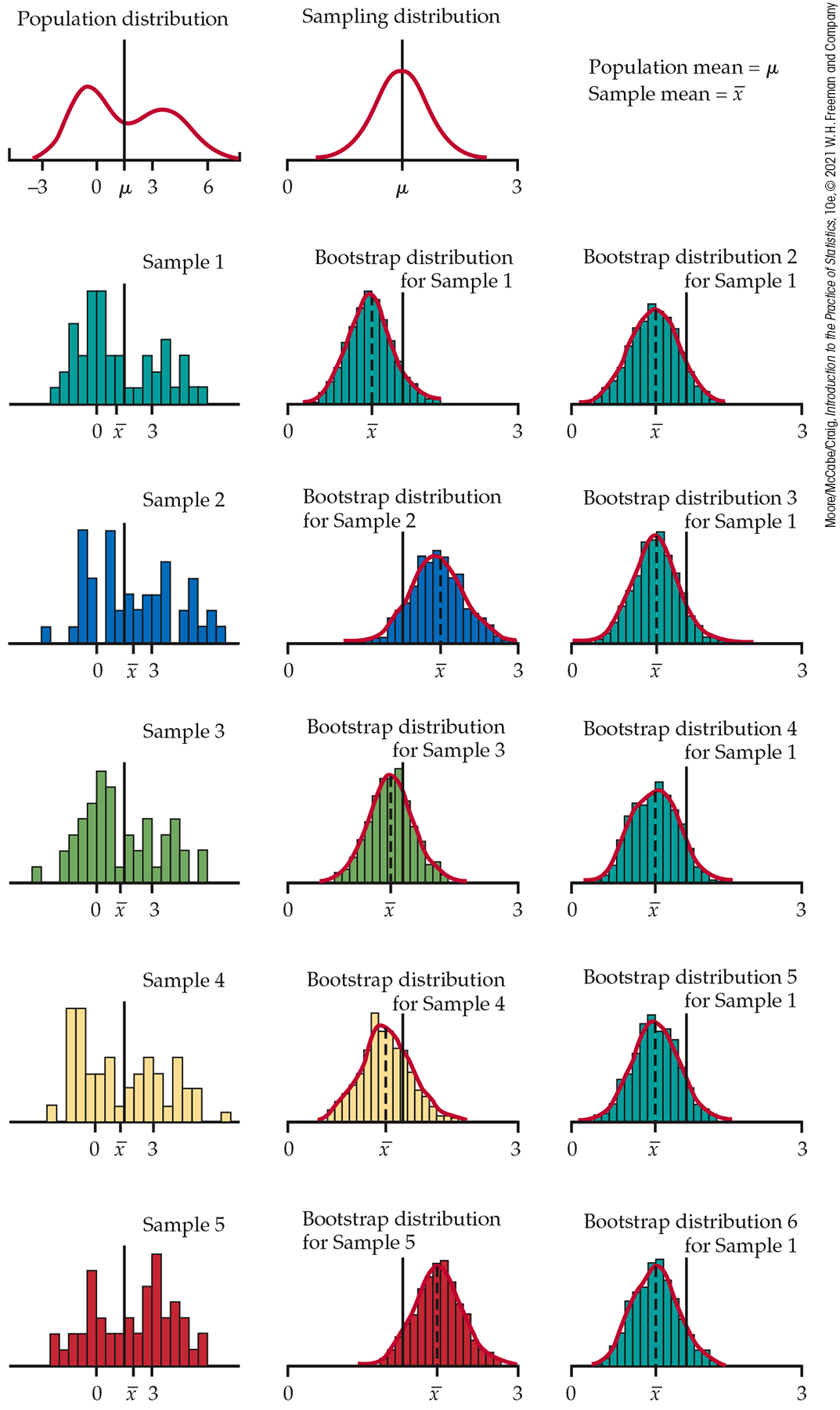
Figure 16.16 shows an example of the entire process. The population distribution (top left) has two peaks and is far from Normal. The histograms in the left column of the figure show five SRSs from this population, each of size 50. The line in each histogram marks the mean x¯ of that sample. The means vary from sample to sample. The distribution of the x¯-values from all possible samples is the sampling distribution. This sampling distribution appears to the right of the population distribution. It is close to Normal, as we expect because of the central limit theorem.

Examples of sampling distributions and bootstrap distributions for five samples. — Figure 16.16 Five random samples of n=50 from the same population, with a bootstrap distribution of the sample mean formed by resampling from each of the five samples. At the right are five more bootstrap distributions from the first sample.

A population distribution curve is shown. It has two peaks, the first higher and the second lower, and a mean of mu. Next to it, a sampling distribution curve is shown. It is normal with mean mu. Fifteen histograms are shown in three columns of five each. The first column shows histograms for five samples, the second shows bootstrap distributions for the same samples, and the third shows five additional bootstrap distributions for sample 1. For sample 1, the sample distribution has two peaks with mean x bar just to the left of the population mean, mu. The bootstrap distribution is roughly normal with mean x bar slightly farther left from mu. The five additional bootstrap distributions each show a roughly normal distribution with nearly identical means to the left of mu. For sample 2, the sample distribution has two peaks with mean x bar just to the right of mu. The bootstrap distribution is roughly normal with mean x bar farther right from mu. For sample 3, the sample distribution has two peaks, with mean x bar nearly equal to mu, but just left of it. The bootstrap distribution is roughly normal with mean x bar just left of mu. For sample 4, the sampling distribution has two peaks, with mean x bar at mu. The bootstrap distribution is roughly normal with x bar a few increments left of mu. For sample 5, the sampling distribution has two peaks, with mean x bar just right of mu. The bootstrap distribution is roughly normal, with mean x bar farther right from mu.

The middle column in Figure 16.16 displays the bootstrap distribution of x¯ for each of the five samples. Each distribution was created by drawing 1000 resamples from the original sample, calculating x¯ for each resample, and presenting the 1000 x¯’s in a histogram. The right column shows the bootstrap distribution of the first sample, repeating the resampling five more times.

Compare the five bootstrap distributions in the middle column to see the effect of the random choice of the original sample. Compare the six bootstrap distributions drawn from the first sample to see the effect of the random resampling. Here’s what we see:

Each bootstrap distribution is centered close to the value of x¯ for its original sample. That is, the bootstrap estimate of bias is small in all five cases. Of course, the five x¯-values vary, and not all are close to the population mean μ.
The shape and spread of the bootstrap distributions in the middle column vary a bit, but all five resemble the sampling distribution in shape and spread. That is, the shape and spread of a bootstrap distribution depend on the original sample, but the variation from sample to sample is not great.
The six bootstrap distributions from the same sample are very similar in shape, center, and spread. That is, random resampling adds very little variation to the variation due to the random choice of the original sample from the population.

Figure 16.16 reinforces facts that we have already relied on. If a bootstrap distribution is based on a moderately large sample from the population, its shape and spread don’t depend heavily on the original sample and do mimic the shape and spread of the sampling distribution. Bootstrap distributions do not have the same center as the sampling distribution; they mimic bias, not the actual center.

The figure also illustrates a fact that is important for practical use of the bootstrap: the bootstrap resampling process (using 1000 or more resamples) introduces very little additional variation. We can rely on a bootstrap distribution to inform us about the bias of the estimate and the shape and spread of the sampling distribution.

Bootstrapping small samples

We now know that almost all the variation in bootstrap distributions for a statistic such as the mean comes from the random selection of the original sample from the population. We also know that, in general, larger samples are preferred because small samples give more variable results. This general fact is also true for bootstrap procedures.

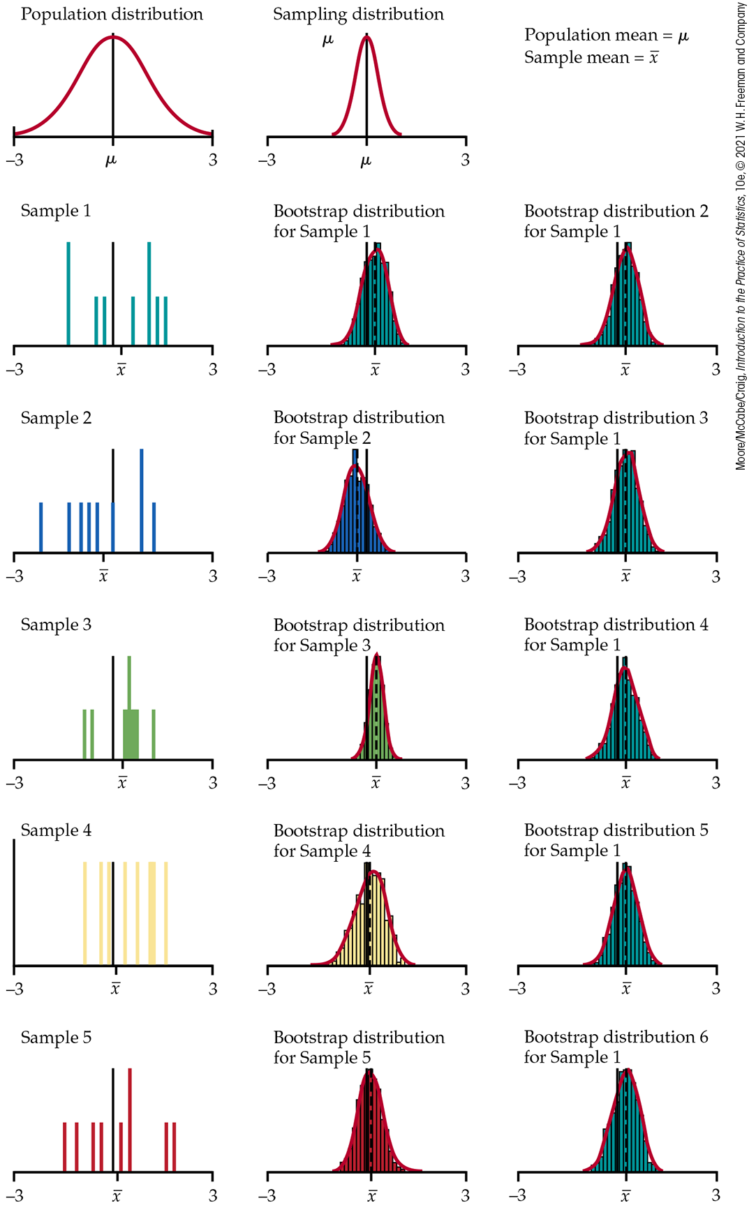
Figure 16.17 repeats Figure 16.16, with two important differences. The five original samples are only of size n=9 rather than the n=50 of Figure 16.16. Also, the population distribution (top left) is Normal, so that the sampling distribution of x¯ is Normal, despite the small sample size.

A population distribution curve is shown. It is roughly normal with mean mu. Next to it, a sampling distribution curve is shown. It is normal, but narrower, with mean mu. Fifteen histograms are shown in three columns of five each. The first column shows histograms for five samples, the second shows bootstrap distributions for the same samples, and the third shows five additional bootstrap distributions for sample 1. For sample 1, the sample distribution has two peaks with mean x bar just to the right of the population mean, mu. The bootstrap distribution is roughly normal with approximately the same mean of x bar just right from mu. The five additional bootstrap distributions each show a roughly normal distribution with nearly identical means to the right of mu. For sample 2, the sample distribution is left skewed with mean x bar just to the left of mu. The bootstrap distribution is roughly normal with approximately the same mean of x bar just left from mu. For sample 3, the sample distribution is slightly left skewed with mean x bar just right of mu. The bootstrap distribution is roughly normal, but narrower than that of sample 2, with approximately the same mean of x bar just right of mu. For sample 4, the sampling distribution is uniform with mean x bar nearly equal to mu, but just to the right. The bootstrap distribution is roughly normal with mean x bar at mu. For sample 5, the sampling distribution is left skewed with mean x nearly equal to x bar, but just to the right. The bootstrap distribution is roughly normal, with mean x bar at mu.

Even with a Normal population distribution, the bootstrap distributions in the middle column show much more variation in shape and spread than those for larger samples in Figure 16.16. Notice, for example, how the skewness of the fourth sample produces a skewed bootstrap distribution. The bootstrap distributions are no longer all similar to the sampling distribution at the top of the column.

caution We can’t trust a bootstrap distribution from a very small sample to closely mimic the shape and spread of the sampling distribution. Bootstrap confidence intervals will sometimes be too long or too short or too long in one direction and too short in the other. The six bootstrap distributions based on the first sample are again very similar. Because we used 1000 resamples, resampling adds very little variation. There are subtle effects that can’t be seen from a few pictures, but the main conclusions are clear.

Bootstrapping a sample median

In dealing with the grade point averages in Example 16.5, we chose to bootstrap the 25% trimmed mean rather than the median. We did this in part because the usual bootstrapping procedure doesn’t work well for the median unless the original sample is quite large. Now we will bootstrap the median in order to understand the difficulties.

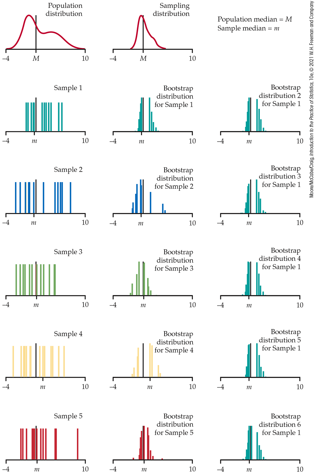
Figure 16.18 follows the format of Figures 16.16 and 16.17. The population distribution appears at top left, with the population median M marked. Below in the left column are five samples of size n=15 from this population, with their sample medians m marked. Bootstrap distributions of the median based on resampling from each of the five samples appear in the middle column. The right column again displays five more bootstrap distributions from resampling the first sample. The six bootstrap distributions from the same sample are, once again, very similar to each other—resampling adds little variation—so we concentrate on the middle column in the figure.

A population distribution curve is shown. It has two peaks, the first higher and the second lower, and a median of upper M. Next to it, a sampling distribution curve is shown. It also has two peaks and median upper M, but is narrower with less spread. Fifteen histograms are shown in three columns of five each. The first column shows histograms for five samples, the second shows bootstrap distributions for the same samples, and the third shows five additional bootstrap distributions for sample 1. For sample 1, the sample distribution is uniform with median lower m just left of the population median upper M. The bootstrap distribution is roughly normal, but with a large gap between its highest bar and the next. It has the same median lower m, to the left of the gap. The five additional bootstrap distributions each show similar distributions. For sample 2, the sample distribution is uniform with median lower m just left of the population median upper M and a wider spread than sample 1. The bootstrap distribution is roughly normal, but with a large gap between its highest bar and the next. It has the same median lower m, to the left of the gap. For sample 3, the sample distribution is uniform with median lower m equal to upper M and a narrower spread than sample 2. The bootstrap distribution is roughly normal, but with a large gap between its highest bar and the next. It has the same median lower m, to the right of the gap. For sample 4, the sample distribution is uniform with median lower m to the right of the population median upper M and a wider spread than sample 3. The bootstrap distribution is roughly normal, but with a large gap between its highest bar and the next. It has the same median lower m, to the right of the gap, with upper M in the gap. For sample 5, the sample distribution is uniform with median lower m equal to upper M and a narrower spread than sample 4, with an outlier to the far right. The bootstrap distribution is roughly normal, but with a large gap between its highest bar and the next. It has the same median lower m, to the left of the gap, with upper M in the gap.

Bootstrap distributions from the five samples differ markedly from each other and from the sampling distribution at the top of the column. Here’s why. The median of a resample of size 15 is the eighth-largest observation in the resample. This is always one of the 15 observations in the original sample and is usually one of the middle observations. Each bootstrap distribution repeats the same few values, and these values depend on the original sample. The sampling distribution, on the other hand, contains the medians of all possible samples and is not confined to a few values.

The difficulty is somewhat less when n is even because the median is then the average of two observations. It is much less for moderately large samples—say n=100 or more. Bootstrap standard errors and confidence intervals from such samples are reasonably accurate, though the shapes of the bootstrap distributions may still appear odd. You can see that the same difficulty will occur for small samples with other statistics, such as quartiles, that are calculated from just one or two observations from a sample.

There are more advanced variations of the bootstrap idea that improve performance for small samples and for statistics such as the median and quartiles. caution Unless you have expert advice or undertake further study, avoid bootstrapping the median and quartiles unless your sample is rather large.

Section 16.3 SUMMARY

Almost all the variation in a bootstrap distribution for a statistic is due to the selection of the original random sample from the population. Resampling introduces little additional variation.
Bootstrap distributions based on small samples can be quite variable. Their shape and spread reflect the characteristics of the sample and may not accurately estimate the shape and spread of the sampling distribution. Bootstrap inference from a small sample may therefore be unreliable.
Bootstrap inference based on samples of moderate size is unreliable for statistics like the median and quartiles that are calculated from just a few of the sample observations.

Section 16.3 EXERCISES

16.28 Variation in the bootstrap distributions. Consider the variation in the bootstrap for each of the following situations with two scenarios, S1 and S2. In comparing the variation, do you expect, in general, that S1 will have less variation than S2, that S2 will have less variation than S1, or that the variation for S1 and S2 will be approximately the same? Give reasons for your answers. Here, we use n for the size of the original sample and B for the number of resamples.
1. S1: n=50, B=2000; S2: n=50, B=4000.
2. S1: n=10, B=2000; S2: n=50, B=2000.
3. S1: n=50, B=200; S2: n=50, B=2000.
4. S1: n=10, B=2000; S2: n=50, B=4000.
16.29 Bootstrap versus sampling distribution. Most statistical software includes a function to generate samples from Normal distributions. Set the mean to 26 and the standard deviation to 27. You can think of all the numbers that would be produced by this function if it ran forever as a population that has the N(26, 27) distribution. Samples produced by the function are samples from this population.
1. What is the exact sampling distribution of the sample mean x¯ for a sample of size n from this population?
2. Draw an SRS of size n=10 from this population. Bootstrap the sample mean x¯ using 2000 resamples from your sample. Give a histogram of the bootstrap distribution and the bootstrap standard error.
3. Repeat the same process for samples of sizes n=40 and n=160.
4. Write a careful description comparing the three bootstrap distributions and also comparing them with the exact sampling distribution. What are the effects of increasing the sample size?
16.30 The effect of increasing the sample size. Refer to the data in Exercise 16.9 (page 16-11). Let’s think of the times from the 187 countries as the population for this exercise. This means the population distribution of times is very non-Normal with one outlier.
1. Find the mean μ and the standard deviation σ for this population.
2. Although we don’t know the shape of the sampling distribution of the sample mean x¯ for a sample of size n from this population, we do know the mean and standard deviation of this distribution. What are they?
3. Draw an SRS of size n=10 from this population. Bootstrap the sample mean x¯ using 2000 resamples from your sample. Give a histogram of the bootstrap distribution and the bootstrap standard error.
4. Repeat the same process for samples of sizes n=40 and n=160.
5. Write a careful description comparing the three bootstrap distributions. What are the effects of increasing the sample size?
16.31 The effect of non-Normality. The populations in the two previous exercises have the same mean and standard deviation, but one is Normal, and the other is strongly non-Normal. Based on your work in these exercises, how does non-Normality of the population affect the bootstrap distribution of x¯? How does it affect the bootstrap standard error? Do either of these effects diminish when we start with a larger sample? Would either of these effects diminish if we considered a larger number of bootstrap resamples? Explain what you have observed based on what you know about the sampling distribution of x¯ and the way in which bootstrap distributions mimic the sampling distribution.