16.1 The Bootstrap Idea
Here is the example we will use to introduce the bootstrap approach.
Example 16.1 Average time looking at a Facebook profile.
![]()
In Example 12.18 (page 624), we compared the amount of time a Facebook user spends reading different types of profiles. Here, let’s focus on just the average time for the fourth profile (negative male). Figure 16.1 gives a histogram and Normal quantile plot of the 21 observations. The data are skewed to the right. Given the relatively small sample size, we have some concerns about using the t confidence interval procedures for these data.
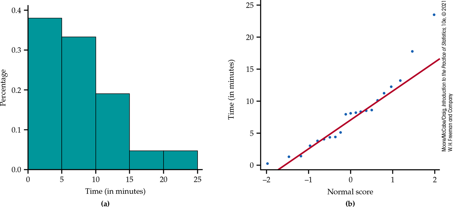
Figure 16.1 Histogram and Normal quantile plot of the distribution of viewing times (in minutes) looking at a negative male Facebook profile page, Example 16.1. The data are right skewed.
The big idea: Resampling and the bootstrap distribution
Statistical inference is based on the sampling distributions of sample statistics. A sampling distribution is based on many random samples from the population. The bootstrap is a way of finding the sampling distribution—at least approximately—from just one sample. We first encountered the bootstrap in Chapter 7 (pages 403–404) when discussing nonparametric procedures. Here is a summary of the method in terms of our Facebook profile example:
Step 1: Resampling. In Example 16.1, we have just one simple random sample (SRS) of 21 cases. In place of many samples from the population, create many resamples by repeatedly sampling with replacement cases from this one SRS. Each resample is the same size as the original SRS.
Sampling with replacement means that after we randomly draw a case from the original sample, we put it back before drawing the next case. Think of drawing a number from a hat and then putting it back before drawing from the hat again. As a result, any number in the hat can be drawn more than once. If we sampled without replacement, we’d get the same set of numbers we started with, though in a different order. Figure 16.2 illustrates three resamples from an SRS of five cases. In practice, we draw hundreds or thousands of resamples, not just three.
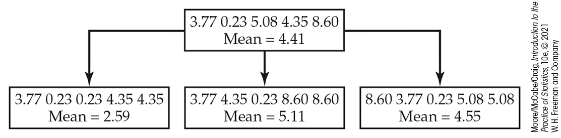
Figure 16.2 The resampling idea. The top box is an SRS of size
Step 2: Bootstrap distribution. The sampling distribution of a statistic describes the values taken by the statistic in all possible samples of the population of the same size. The bootstrap distribution of a statistic summarizes the values taken by the statistic in all possible resamples of the same size. The bootstrap distribution gives information (i.e., shape and spread) about the sampling distribution.
Example 16.2 Bootstrap distribution of the mean time looking at a Facebook profile.
![]()
In Example 16.1, we want to estimate the average viewing time of a negative male Facebook profile
We randomly generated 3000 resamples for these data. The mean for the resamples is 7.89 minutes, and the standard deviation is 1.22 minutes. Figure 16.3(a) gives a histogram of the bootstrap distribution of the means of 3000 resamples from the viewing time data. The Normal density curve with the mean 7.89 and standard deviation 1.22 is superimposed on the histogram. A Normal quantile plot is given in Figure 16.3(b). The Normal curve fits the data well, but some skewness is still present.
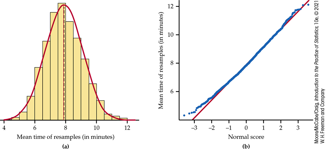
Figure 16.3 (a) The bootstrap distribution of 3000 resample means from the sample of Facebook profile viewing time data. The smooth curve is the Normal density function for the distribution, which matches the mean and standard deviation of the distribution of the resample means. (b) The Normal quantile plot confirms that the bootstrap distribution is slightly skewed to the right but fits the Normal distribution quite well.
According to the bootstrap idea, the bootstrap distribution represents the sampling distribution.
Example 16.3 Assessing the bootstrap distribution.
Let’s compare the bootstrap distribution with what we know about the sampling distribution of
Shape: We see that the bootstrap distribution is nearly Normal. The central limit theorem says that the sampling distribution of the sample mean
Center: The bootstrap distribution is centered close to the mean of the original sample, 7.89 minutes versus 7.87 minutes for the original sample. Therefore, the mean of the bootstrap distribution has little bias as an estimator of the mean of the original sample. We know that the sampling distribution of
Spread: The histogram and density curve in Figure 16.3(a) picture the variation among the resample means. We can get a numerical measure by calculating their standard deviation. Because this is the standard deviation of the 3000 values of
The bootstrap standard error 1.22 is close to the theory-based estimate 1.23.
In discussing Example 16.2, we used statistical theory to describe the sampling distribution of the sample mean
The great advantage of the resampling idea is that it often works in settings when theory does not apply. Of course, theory also has its advantages: we know exactly when it works. We don’t know exactly when resampling works, so that “When can I safely bootstrap?” is a somewhat subtle issue (see Section 16.3).
Figure 16.4 illustrates the bootstrap idea by comparing three distributions. Figure 16.4(a) shows the idea of the sampling distribution of the sample mean
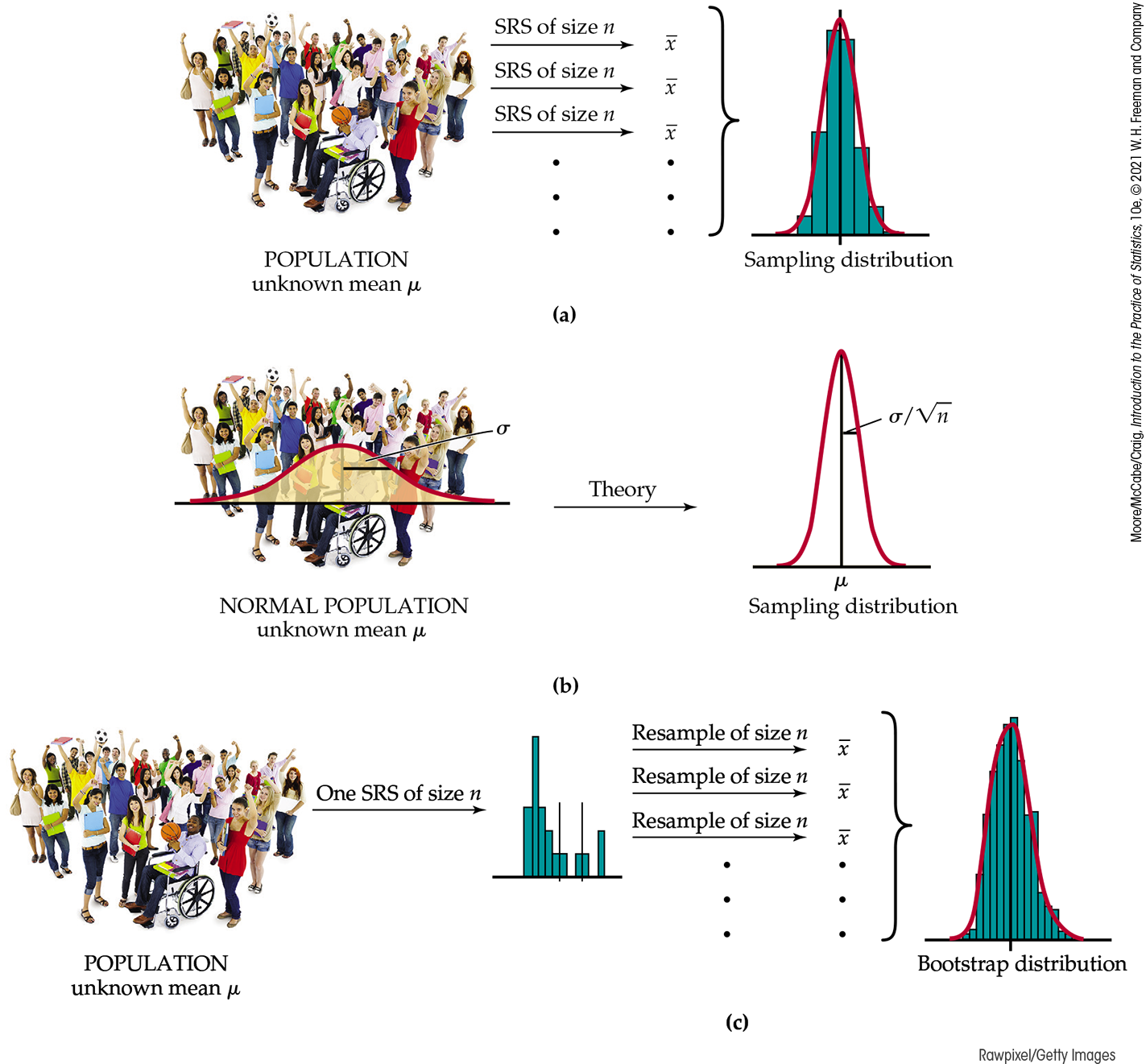
Figure 16.4 (a) The idea of the sampling distribution of the sample mean
Figure 16.4(b) shows how traditional inference works: statistical theory tells us that if the population has a Normal distribution, then the sampling distribution of
Figure 16.4(c) shows the bootstrap idea: we avoid the task of taking many samples from the population by instead taking many resamples from a single sample. The values of
Check-in
16.1 A small bootstrap example. To illustrate the bootstrap procedure, let’s bootstrap a small random subset of the Facebook profile data:

Sample with replacement from this initial SRS by rolling a die. Rolling a 1 means select the first member of the SRS, a 2 means select the second member, and so on. (You can also use Table B of random digits and respond only to digits 1 to 6.) Create 20 resamples of size
Calculate the sample mean for each of the resamples.
Make a stemplot of the means of the 20 resamples. This is an estimate of the bootstrap distribution.
Calculate the bootstrap standard error.
16.2 Standard deviation versus standard error. Explain the difference between the standard deviation of a sample and the standard error of a statistic such as the sample mean.
Thinking about the bootstrap idea
It might appear that resampling creates new data out of nothing. Even the name “bootstrap” comes from the impossible image of “pulling yourself up by your own bootstraps.”2 However, the resamples are not used as if they were new data. The bootstrap distribution of the resample means is used only to estimate how the sample mean of one actual sample of size 21 would vary because of random sampling.
Using the same data for two purposes—to estimate a parameter and also to estimate the variability of the estimate—is perfectly legitimate. We do exactly this when we calculate
What is new? First of all, we don’t rely on the formula
To make clear that these are the mean and standard deviation of the means of the B resamples rather than the mean
These formulas go all the way back to Chapter 1. Once we have the values
Because we will often apply the bootstrap to statistics other than the sample mean, here is the general definition for the bootstrap standard error.
Second, we don’t appeal to the central limit theorem or other theory to tell us that a sampling distribution is roughly Normal. We simply look at the bootstrap distribution using the methods of Chapter 1 to see if it is roughly Normal (or not). What we find determines how to proceed in constructing a confidence interval.
In summary, the bootstrap allows us to calculate standard errors for statistics for which we don’t have formulas and to check Normality of the sampling distribution for statistics that theory doesn’t easily handle. To apply the bootstrap idea, we must start with a statistic that estimates the parameter we are interested in. We come up with a suitable statistic by appealing to another principle that we have often applied without thinking about it.
This principle tells us to estimate a population mean
Using software
Software is essential for bootstrapping in practice. Here is an outline of the program you would write if your software can choose random samples from a set of data but does not have bootstrap functions:
Repeat B timesDraw a resample with replacement from the data.Calculate the resample statistic.Save the resample statistic into a variable.
Make a histogram and Normal quantile plot of the B resample statistics.Calculate the mean and standard deviation of the B statistics.
Example 16.4 Using software.
![]()
R has packages that contain various bootstrap functions, so we do not have to write them ourselves. If the 21 viewing times are saved as a variable, we can use functions to resample from the data, calculate the means of the resamples, and request both graphs and printed output. We can also ask that the bootstrap results be saved for later access.
The function plot within the package boot will generate graphs similar to those in Figure 16.3 so you can assess Normality. Figure 16.5 contains the default output from a call of the function boot. The variable Time contains the 21 viewing times, the function theta is specified to be the mean, and we request 3000 resamples. The original entry gives the mean Bias is the difference between the mean of the resample means and the original mean. If we add the entries for bias and original, we get the mean of the resample means,
The bootstrap standard error is displayed under std. error. All these values except original will differ slightly if you take another 3000 resamples because the resamples are drawn at random.
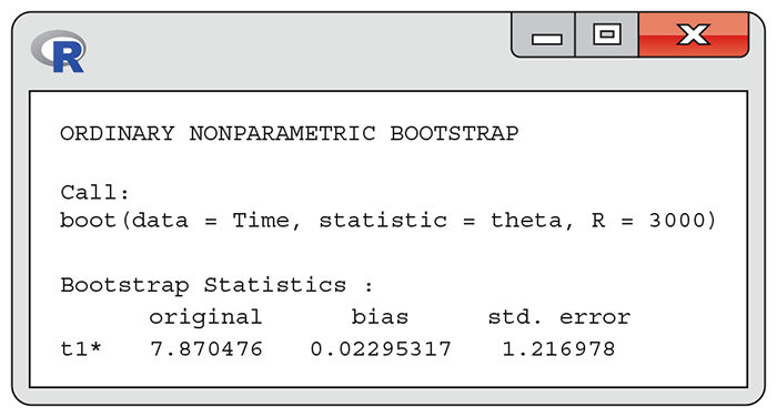
Figure 16.5 R output of the bootstrap applied to the Facebook profile viewing time data, Example 16.3.
Section 16.1 SUMMARY
To bootstrap a statistic such as the sample mean, draw with replacement hundreds or thousands of resamples of the same size from a single original sample and calculate the statistic for each resample. This collection of resample statistics approximates the bootstrap distribution, which summarizes the values of all possible resample statistics from the single original sample.
A bootstrap distribution approximates the sampling distribution of the statistic, usually sharing the same shape and spread. It is centered at the statistic (from the original sample) when the sampling distribution is centered at the parameter (of the population). The bootstrap standard error is the standard deviation of the bootstrap distribution.
Use graphical and numerical summaries to determine whether the bootstrap distribution is approximately Normal and centered at the original statistic and to assess its spread. This information is used to determine the appropriate bootstrap confidence interval.
If we take B resamples and call the means of these resamples
The bootstrap standard error of
Using the sample mean to estimate the population mean is an example of the plug-in principle: use a quantity based on the sample to approximate a similar quantity from the population.
Section 16.1 EXERCISES
16.1 What’s wrong? For each of the following, explain what is wrong and why.
The standard deviation of the bootstrap distribution will be approximately the same as the standard deviation of the original sample.
The bootstrap distribution is created by resampling without replacement from the original sample.
When generating the resamples, it is best to use a sample size smaller than the size of the original sample.
The bootstrap distribution is created by resampling with replacement from the population.
16.2 Describing the method to obtain resamples. Suppose an SRS of size
16.3 Gosset’s data on double stout sales. William Sealy Gosset worked at the Guinness Brewery in Dublin and made substantial contributions to the practice of statistics. In Exercise 1.37 (page 44), we examined Gosset’s data on the change in the double stout market before and after World War I (1914–1918). Here are the data for a sample of six of the regions in the original data:

Bristol 94 Glasgow 66 English P 46 Liverpool 140 English Agents 78 Scottish 24 Do you think that these data appear to be from a Normal distribution? Give reasons for your answer.
Select five resamples from this set of data, making sure to describe how this sampling was performed.
Compute the mean for each resample.
Find the bootstrap standard error.
16.4 More on the bootstrap standard error. Refer to your work in the previous exercise.
Do you expect your bootstrap standard error to be larger, smaller, or approximately equal to the standard deviation of the original sample of six regions? Explain your answer.
Would your answer change if the bootstrap standard error were based on 500 resamples instead of 5? Explain your answer.
16.5 Assessing the bootstrap distribution. Refer to the data in Exercise 16.3. Figure 16.6 gives a histogram and a Normal quantile plot of 3000 resample means (labeled t*). What do these plots tell you about the sampling distribution of
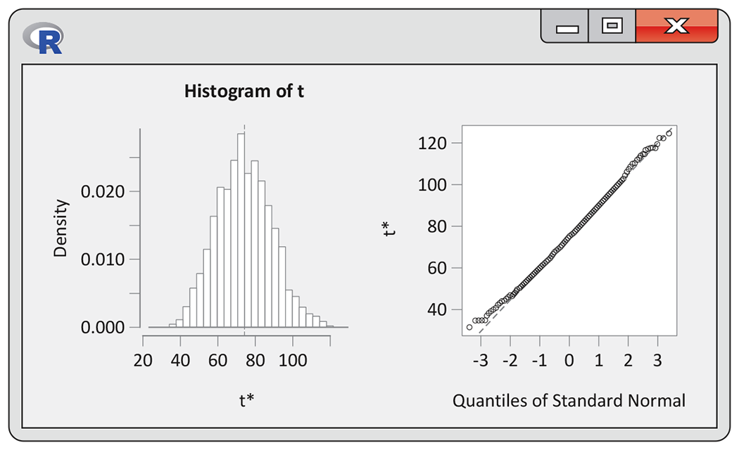
Figure 16.6 R graphical output for the percent change in double stout sales bootstrap, Exercise 16.5.
16.6 Assessing another bootstrap distribution. Refer to the data in Check-in question 16.1 (page 16-6). Figure 16.7 gives a histogram and a Normal quantile plot of 3000 resample means (labeled t*). What do these plots tell you about the sampling distribution of
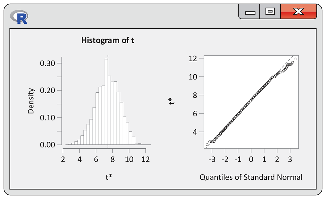
Figure 16.7 R graphical output for the Facebook viewing time bootstrap, Exercise 16.6.
16.7 Interpreting the output. Figure 16.8 gives output from R for the sample of ratios (as a percent) in Exercise 16.3. Summarize the results of the analysis using this output.
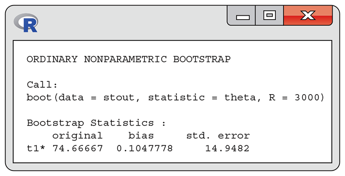
Figure 16.8 R output for the percent change in double stout sales bootstrap, Exercise 16.7.
16.8 Interpreting bootstrap output. Figure 16.9 gives output from R for the sample of six viewing times in Check-in question 16.1 (page 16-6). Summarize the results of the analysis using this output.
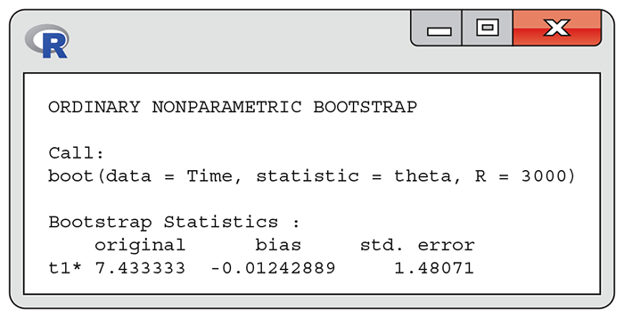
Figure 16.9 R output for the Facebook viewing time bootstrap, Exercise 16.8.
Inspecting the bootstrap distribution of a statistic helps us judge whether the sampling distribution of the statistic is close to Normal. For each of the data sets in Exercises 16.9 through 16.12, determine whether you’d be comfortable using inference methods that rely of Normality by bootstrapping the sample mean
16.9 Bootstrap distribution of the time to start a business. We examined the distribution of the time to start a business for 187 countries in Example 1.43 (page 60). The distribution is clearly skewed and has an outlier. We view these data as coming from a process that gives times to start a business around the globe.

16.10 Bootstrap distribution of average IQ score. The distribution of the 60 IQ test scores in Table 1.1 (page 15) is roughly Normal (see Figure 1.7), and the sample size is large enough that we expect a Normal sampling distribution.

16.11 Bootstrap distribution of delivery time from COSI. A random sample of eight times (in minutes) it took a delivery robot to bring you lunch from COSI to your dormitory (Example 7.1, page 387) are
The distribution has no outliers, but we cannot comfortably assess Normality from such a small sample.

16.12 Bootstrap distribution of average audio file length. The lengths (in seconds) of audio files found on an iPod (Table 7.3, page 399) are skewed. We previously transformed the data prior to using t procedures.

16.13 Standard error versus the bootstrap standard error. We have two ways to estimate the standard deviation of a sample mean
Find the sample standard deviation s for the 60 IQ test scores in Exercise 16.10 and use it to find the standard error
Find the sample standard deviation s for the time to start a business data in Exercise 16.9 and use it to find the standard error

Find the sample standard deviation s for the eight delivery times in Exercise 16.11 and use it to find the standard error
16.14 Visit lengths to a statistics help room. Table 5.1 (page 283) gives the length (in minutes) for a sample of 50 visits to a statistics help room. See Example 5.5 (page 283) for more details about these data.

Make a histogram of the 50 visit lengths. Describe the shape. Is it similar to the distribution of all 1264 recorded visits?
The central limit theorem says that the sampling distribution of the sample mean
16.15 More on help room visit lengths. Here is an SRS of 10 of the visit lengths from Exercise 16.14:

We expect the sampling distribution of
Create and inspect the bootstrap distribution of the sample mean for these data using 1000 resamples. Compared with your distribution from the previous exercise, is this distribution closer to or farther away from Normal?
Compare the bootstrap standard errors for your two sets of resamples. Why is the standard error larger for the smaller SRS?