16.1 Answers will vary.

16.3

1. Answers will vary based on the mean calculated in 16.1.
2. 1.20.
3. (5.34, 10.34).

16.5

1. Based on 2000 resamples, SEboot is almost always between 3.9 and 4.5.
2. The bootstrap distribution looks reasonably Normal, with a little bias.
3. The t interval is 1.2 to 18.7.

16.7

1. For the 99% bootstrap percentile confidence interval, there is 0.5% on either end, so we need the 0.5 percentile and 99.5 percentile. For the 90% bootstrap percentile confidence interval, we need the 5th percentile and the 95th percentile.

16.9 No, because we believe that one population has a smaller variability. In order to pool the data, the permutation test requires that both populations be the same when H0 is true.

16.1

1. The standard deviation of the bootstrap distribution will be approximately s/n.
2. Bootstrap samples are done with replacement from the original sample.
3. You should use a sample size equal to the original sample size.
4. The bootstrap distribution is created by sampling with replacement from the original sample, not the population.

16.3

1. Answers will vary, but a Normal quantile plot indicates that it is roughly Normal.
2. Answers will vary.
3. The means could range from 24 to 140, but based on 2000 resamples, the means should range between 33 and 122.
4. Answers will vary, but based on 2000 sets of five bootstrap samples, the error should vary between 3.5 and 28.8.

16.5 The sampling distribution is approximately Normal, with the mean of the bootstrap distribution around 78.

16.7 The mean of the original sample is 74.6667; the mean of the bootstrap distribution is 0.1047778 higher. The bootstrap standard error is 14.9482.

16.9 The bootstrap appears Normal.

16.11 The bootstrap appears Normal.

16.13 The bootstrap standard errors will vary.

16.15

1. The larger resamples are closer to Normal.
2. The standard error is larger for the smaller SRS because with the smaller sample sizes, there is more variability.

16.17

1. We use the bootstrap t interval when the bias is small, not when it is large.
2. Here, we can use the bootstrap t interval.

• (c–d) Do not use the bootstrap t interval when the bootstrap distribution is clearly skewed.

16.19

1. Answers will vary.

16.21

1. The bootstrap distribution looks reasonably Normal.
2. (51.1169, 73.0831).
3. σ/n=5.465. The two confidence intervals are very close.

16.23 The bootstrap distribution of the standard deviation looks quite Normal. This particular resample had SEboot=0.0489 and mean 0.814. The original sample of GPAs had s=0.817, so there is little bias. With n=150, we can use df=100, t*=1.984 and find a 95% confidence interval for the population standard deviation of 0.7200 to 0.9140.

16.25

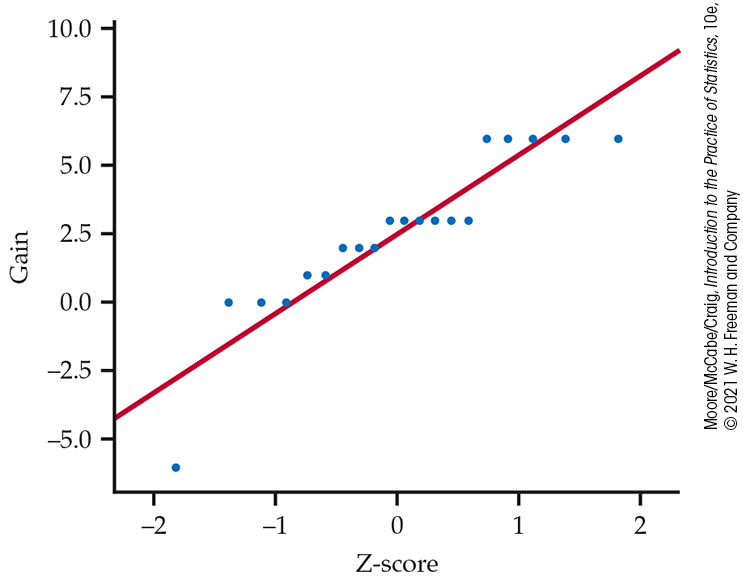
1. The data appear to be roughly Normal though with the typical random gaps and bunches that usually occur with relatively small samples. It appears from both the histogram and quantile plot that the mean is slightly larger than zero, but the difference is not large enough to rule out the N(0,1) distribution.
2. The bootstrap distribution is extremely close to Normal, with no appreciable bias.
3. The typical SE is 0.1308, and the t interval is −0.1357 to 0.3854.

16.27

1. s=1.4841.
2. 0.3721.
3. The standard error is much smaller than the standard deviation of the sample.
4. Yes.

16.29

1. The distribution of x¯ is N(26, 27/n).
2. SEboot ranged from about 6.49 to about 7.08.
3. For n=40, the original random sample had s=29.21. SEboot ranged from about 4.2 to 4.7. For n=160, SEboot ranged from about 2.02 to about 2.25.

16.31 Answers will vary.

16.33 The bootstrap distribution is right-skewed; an interval based on t would not be appropriate. The original sample had the statistic of interest θ^=0.6137. The bootstrap distribution had a sample mean a bit higher because the bias is 0.0328. SEboot=0.2433. The BCa confidence interval is (0.2831, 1.1943), which is located about 0.16 higher than the regular bootstrap interval and lower than the percentile interval.

16.35

1. The bootstrap percentile and t intervals are very similar, suggesting that the t intervals are acceptable.
2. Every interval (percentile and t) includes 0.

16.37 The results of the bootstrap interval may have a slightly larger standard error and also may have slightly higher bias.

16.39 One set of 1000 repetitions gave the BCa interval as (0.4503, 0.8049). We see the bootstrap distribution is left-skewed and that there was one possible high outlier as well. The lower end of the BCa interval typically varies between 0.42 and 0.46, while the upper end varies between 0.795 and 0.805. These intervals are lower than those found in the earlier example.

16.43 Answers will vary, but the confidence intervals will be wider with smaller sample sizes.

16.45 Typical ranges for the endpoints of the BCa interval (using males–females) are given below. This interval is comparable to the −0.416 to 0.118 found in Example 16.9.

16.47

1. Answers will vary. The shape is roughly Normal, with a small bias. Simple bootstrap inference can be used.
2. Answers will vary. The confidence intervals should be close.

16.49

1. The regression line is Rating^=26.724+1.207 PricePerLoad.
2. The ends of the bootstrap distribution do not look very Normal; a t interval may not be appropriate.
3. The typical standard error of the slope is 0.2846. With t22=2.074, the typical confidence interval would be 0.6167 to 1.7973. All these intervals seem to be located higher.

16.51

1. The distribution of the slope b1 looks approximately Normal, and the t distribution should be accurate.
2. The bootstrap confidence interval is (−0.23018, −0.2242), and the bootstrap t-value=−149.13.

16.53 Enter the data with the score given to the phone and an indicator for each design. We have hypotheses H0:   μ1=μ2 and Ha:   μ1≠μ2. Resample the design indicators (without replacement) to scramble them. Compute the mean score for each scrambled design group. Repeat the process many times. The P-value of the test will be the proportion of resamples where the resampled difference in group means is larger than the observed difference (in absolute value).

16.55 If there is no relationship, we have H0:   ρ=0. We test this against Ha:   ρ≠0. Because there is no relationship under H0, we can resample one of the variables—say, screen satisfaction (without replacement)—and compute the correlation between that and the original scores for keyboard satisfaction. Repeat the process many times, keeping track of the proportion of resamples where the correlation is greater in absolute value than that found in the original data. That proportion is the P-value for the test.

16.57

1. The observed difference in means is 18.5.

• (b–c) Answers will vary.

4. Out of 20 resamples, the number that yield a difference of 18.5 (or more) have a binomial distribution with n=20 and p=3/15, so students should get between 0 and 8 or 9 resamples that give a value of 18.5 or larger, for a P-value ranging between 0 and 0.45.
5. Only one resample possibility can give a difference of means greater than or equal to the observed value, so the exact P-value is 3/15=0.2.

16.59

1. H0:   μ1=μ2 versus Ha:   μ1≠μ2.
2. t=3.81, P-value=0.0052.
3. P-value=0.0163.
4. Answers will vary.

16.61

1. The two populations should be the same shape but skewed (or otherwise clearly non-Normal) so that the t test is not appropriate.
2. Either test is appropriate if the two populations are both Normal with the same standard deviation.
3. We can use a t test but not a permutation test if both populations are Normal with different standard deviations.

16.63

1. We test H0:   μ=0 versus Ha:   μ>0, where μ is the population mean difference before and after the summer language institute. We find t=3.86, df=19, and P-value=0.0005.
2. The Normal quantile plot (right) looks odd because we have a small sample, and all differences are integers.

3. The P-value is almost always less than 0.002. Both tests lead to the same conclusion: The difference is statistically significant (that is, the language institute did help comprehension).

   

16.65

1. We have H0:   ρ=0 versus Ha:   ρ≠0.
2. The observed correlation is r=0.671. We create permutation samples and observe the proportion with correlations at least 0.671 in absolute value. You should find a P-value 0.002 or less. We’ll conclude that there is a correlation between price and rating for laundry detergents.

16.67 For testing H0: All σi2 are equal versus Ha: At least one σi2 is different, the permutation test P-value will almost always be between 0.65 and 0.68. There is not enough evidence to suggest a difference in variances. In Example 12.17, the P-value=0.6775, which agrees with the permutation test.

16.69 For the permutation test, we must resample in a way that is consistent with the null hypothesis. Hence, we pool the data—assuming that the two populations are the same—and draw samples (without replacement) for each group from the pooled data. For the bootstrap, we do not assume that the two populations are the same, so we sample (with replacement) from each of the two data sets separately rather than pool the data first.

16.71

1. We will test H0:   μ1=μ2 versus Ha:   μ1≠μ2. (Males are coded as 1 in the data file.) The observed mean for males was 2.7835, and the observed mean for females was 2.9325. We seek the proportion of resamples where the absolute value of the difference was at least 0.149. The P-value should generally be between 0.25 and 0.32. This test finds no significant difference in GPA between the two sexes.
2. We test H0:   σ1/σ2=1 versus Ha:   σ1/σ2≠1. The observed ratio is 1.149. The P-value is generally between 0.235 and 0.270. We fail to detect a difference in the standard deviations of GPAs for males and females.

16.73 The 95% t interval is narrower in some cases than the percentile interval. In Example 16.8, the percentile interval was 2.793 to 3.095 (a bit narrower and higher than the bootstrap confidence intervals), and the t interval was 2.80 to 3.10 (again, narrower and higher). This is at least in part explained by eliminating more observations on either end with the 25% trim.

16.75

1. The correlation for males is 0.4657. Because the bootstrap distribution does not look Normal, we focus on the percentile interval. The lower end of the percentile intervals ranged from 0.269 to 0.286, with the upper end ranging from 0.623 to 0.625.
2. The correlation for females is 0.3649. Again focusing on the percentile interval, the intervals are wider. The low end of the percentile interval ranged from 0.053 to 0.081, while the upper end ranged from 0.581 to 0.604.
3. The plot shows that the bootstrap distribution of the differences in correlations is very Normal. It is also clear that 0 will be included in the interval; the interval for this bootstrap set was (−0.2426, 0.4229). All intervals examined had a low end between −0.22 and −0.24 and a high end between 0.40 and 0.42. We can conclude that there is no significant difference in the correlation between high school math grades and college GPA by gender.

16.77 The bootstrap distribution looks quite Normal, and (as a consequence) all of the bootstrap confidence intervals are similar to each other and also are similar to the standard (large-sample) confidence interval.

16.79

1. There were 32 poets who died at an average age of 63.19 years (s=17.30), with median age 68. There were 24 nonfiction writers, who died at an average age of 76.88 years (s=14.10), with median age 77.5. Side-by-side boxplots clearly show that poets seem to die younger. Both distributions are somewhat left-skewed, and the nonfiction writer who died at age 40 is a low outlier.
2. Using a two-sample t test, we find that testing H0:   μN=μP against Ha:   μN≠μP gives t=3.26 with P-value=0.002(df=53). A 95% confidence interval for the difference in mean ages is (5.27, 22.11). Nonfiction writers seem to live, on average, between 5.27 and 22.11 years longer than poets, at 95% confidence.
3. The bootstrap distribution is symmetric and seems close to Normal, except at the ends of the distribution, so a bootstrap t interval should be appropriate. The low ends of the bootstrap interval are typically between 5.26 and 5.82; the high ends are typically between 21.26 and 22.15. One particular interval seen was (5.40, 21.36). Note that this interval is a bit narrower than the two-sample t interval.

16.81 The R permutation test for the mean ages returns a P-value of 0.006 (comparable to the 0.002 from the t test) in this instance. The 99% confidence interval for the P-value is between 0.0002 and 0.0185. We can determine that there is a difference in mean age at death between poets and nonfiction writers.

16.83 All answers (including the shape of the bootstrap distribution) will depend strongly on the initial sample of uniform random numbers. The median M of these initial samples will be between about 0.36 and 0.64 about 95% of the time; this is the center of the bootstrap t confidence interval.

1. For a uniform distribution of 0 to 1, the population median is 0.5.
2. Most of the time, the bootstrap distribution is quite non-Normal.
3. SEboot typically ranges from about 0.04 to 0.12 (but may vary more than that, depending on the original sample). The bootstrap t interval is, therefore, roughly M±2SEboot.
4. The more sophisticated BCa and tilting intervals may or may not be similar to the bootstrap t interval. The t interval is not appropriate because of the non-Normal shape of the bootstrap distribution and because SEboot is unreliable for the sample median; it depends strongly on the sizes of the gaps between the observations near the middle.

16.85 Answers will vary.

16.87

1. The 33% is the middle value from the confidence interval.

• (b–c) Answers will vary.

16.89

1. The standard test of H0:   σ1=σ2 versus Ha:   σ1≠σ2 leads to F=0.3443 with df 13 and 16; P-value=0.0587.
2. The permutation P-value is typically between 0.02 and 0.03.
3. The P-values are similar, even though, technically, the permutation test is significant at the 5% level, while the standard test is (barely) not. Because the samples are too small to assess Normality, the permutation test is safer. (In fact, the population distributions are discrete, so they cannot follow Normal distributions.)

16.91

1. The mean ratio is 1.0596; the usual t interval is 1.0063 to 1.1128. The bootstrap distribution for the mean is close to Normal, and the bootstrap confidence intervals are usually similar to the usual t interval but slightly narrower. Bootstrapping the median produces a clearly non-Normal distribution; the bootstrap t interval should not be used for the median.
2. The ratio of means is 1.0656; the bootstrap distribution is noticeably skewed, so the bootstrap t is not a good choice, but the other methods usually give intervals similar to 0.75 to 1.55.
3. For example, the usual t interval from part (a) could be summarized by the statement “On average, Jocko’s estimates are 1% to 11% higher than those from other garages.”