16.2 First Steps in Using the Bootstrap
To introduce the key ideas of resampling and bootstrap distributions, we studied an example in which we knew quite a bit about the actual sampling distribution (i.e., the sampling distribution of
The center of the bootstrap distribution is not the same as the center of the sampling distribution. The sampling distribution of a statistic used to estimate a parameter is centered at the actual value of the parameter in the population, plus any bias. The bootstrap distribution is centered at the value of the statistic for the original sample, plus any bias. A key fact is that the two biases are similar in size even though the two centers may differ.
The bootstrap method is most useful in settings where we don’t know the sampling distribution of the statistic. The principles for any statistic are
Shape: Because the shape of the bootstrap distribution approximates the shape of the sampling distribution, we can use the bootstrap distribution to check Normality of the sampling distribution, as we did in Example 16-3 (page 16-5).
Center: A statistic is biased as an estimate of the parameter if its sampling distribution is not centered at the true value of the parameter. We can check bias by seeing whether the bootstrap distribution of the statistic is centered at the value of the statistic for the original sample.
More precisely, the bias of a statistic is the difference between the mean of its sampling distribution and the true value of the parameter. The bootstrap estimate of bias is the difference between the mean of the bootstrap distribution and the value of the statistic in the original sample. The size of this bias is interpreted relative to the size of the statistic and relative to the size of the bootstrap standard error.
Spread: The bootstrap standard error of a statistic is the standard deviation of its bootstrap distribution. The bootstrap standard error estimates the standard deviation of the sampling distribution of the statistic.
Bootstrap t confidence intervals
If the bootstrap distribution of a statistic shows a Normal shape and small bias, we can construct a confidence interval for the parameter by using the bootstrap standard error and the familiar t distribution. We’ll use an example to show how this works.
Example 16.5 Grade point averages.
![]()
A study of college students at a large university looked at grade point average (GPA) after three semesters of college as a measure of success. In Example 11.1 (page 565), we examined predictors of GPA. Let’s take a look at the distribution of the GPA for the 150 students in this study.
A histogram is given in Figure 16.10(a). The Normal quantile plot is given in Figure 16.10(b). The distribution is strongly skewed to the left. The Normal quantile plot suggests that there are several students with perfect (4.0) GPAs and one at or near the lower end of the distribution (0.0). These data are not Normally distributed.
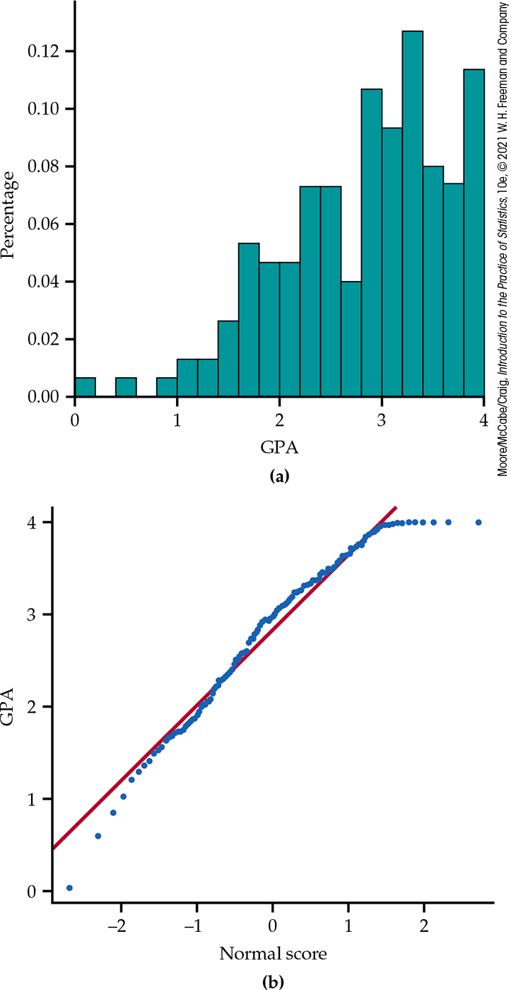
Figure 16.10 Histogram and Normal quantile plot for 150 grade point averages, Example 16.5. The distribution is skewed to the left.
Because of the lack of symmetry, let’s abandon the mean in favor of a statistic that better focuses on the central part of a skewed distribution. We might choose the median, but in this case, we will use the 25% trimmed mean, the mean of the middle 50% of the observations. The median is simply the middle observation or the mean of the two middle observations. Thus, the trimmed mean often does a better job of representing the average of typical observations than does the median.
Our parameter is the 25% trimmed mean of the population of college student GPAs after three semesters at this large university. By the plug-in principle, the statistic that estimates this parameter is the 25% trimmed mean of the sample of 150 students. Because 25% of 150 is 37.5, we drop the 37 lowest and 37 highest GPAs and find the mean of the remaining 76 GPAs. The statistic is
Given the relatively large sample size
Fortunately, we don’t need any distribution facts to use the bootstrap. We bootstrap the 25% trimmed mean just as we bootstrapped the sample mean: draw 3000 resamples of size 150 from the 150 GPAs, calculate the 25% trimmed mean for each resample, and form the bootstrap distribution from these 3000 values.
Example 16.6 Interpreting the bootstrap results.
![]()

Figure 16.11 shows the bootstrap distribution of the 25% trimmed mean. Here is the summary output from R:
ORDINARY NONPARAMETRIC BOOTSTRAPCall:boot(data = GPA, statistic = theta, R = 3000)Bootstrap Statistics : original bias std. error
t1* 2.949605 −0.002912 0.0778597
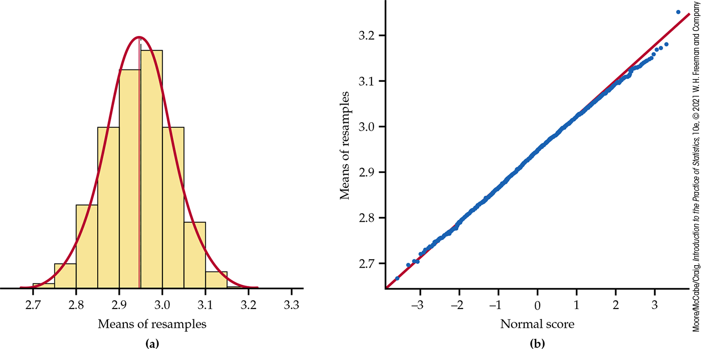
Figure 16.11 The bootstrap distribution of the 25% trimmed means for 3000 resamples from the GPA data in Example 16.6. The bootstrap distribution is approximately Normal.
What do we see?
Shape: The bootstrap distribution is close to Normal. This suggests that the sampling distribution of the trimmed mean is also close to Normal.
Center: The bootstrap estimate of bias is
Spread: The bootstrap standard error of the statistic is
This is an estimate of the standard deviation of the sampling distribution of the trimmed mean.
Recall the familiar one-sample t confidence interval (page 386) for the mean of a Normal population:
This interval is based on the Normal sampling distribution of the sample mean
![]() Note that this interval uses the original value of the statistic, not the mean of the bootstrap distribution.
Note that this interval uses the original value of the statistic, not the mean of the bootstrap distribution.
Example 16.7 Bootstrap t confidence interval of the trimmed mean.
![]()
We want to estimate the 25% trimmed mean of the population of all college student GPAs after three semesters at this large university. We have an SRS of size
Because Table D does not have entries for = T.INV.2T(0.05,75) to get
We are 95% confident that the 25% trimmed mean (the mean of the middle 50%) for the population of college student GPAs after three semesters at this large university is between 2.795 and 3.105.
Check-in
16.3 Bootstrap t confidence interval. Recall Example 16.1 (page 16-3). Suppose a bootstrap distribution is created using 3000 resamples and that the mean and standard deviation of the resample means are 7.84 and 1.20, respectively.
What is the bootstrap estimate of the bias?
What is the bootstrap standard error of
Assume that the bootstrap distribution is reasonably Normal. Because the bias is small relative to the observed
16.4 Bootstrap t confidence interval for average audio file length. Return to or create the bootstrap distribution resamples on the sample mean for audio file length in Exercise 16.12 (page 16-11). In Example 7.10 (page 400), the t confidence interval was applied to both the time lengths and the logarithm of the time measurements.

Inspect the bootstrap distribution. Are the conditions met so that we can use a bootstrap t confidence interval? Explain why or why not.
Construct the 95% bootstrap t confidence interval.
Compare the bootstrap results with the t confidence interval for average time reported in Example 7.10.
Bootstrapping to compare two groups
Two-sample problems are among the most common statistical settings. In a two-sample problem, we wish to compare two populations, such as male and female college students, based on separate samples from each population. When both populations are roughly Normal, the two-sample t procedures compare the two population means.
The bootstrap can also compare two populations, without the Normality condition and without the restriction to a comparison of means. The most important new idea in terms of implementation is that bootstrap resampling must mimic the “separate samples” design that produced the original data.
Example 16.8 Bootstrap comparison of GPAs.
![]()
In Example 16.5, we looked at grade point average (GPA) after three semesters of college as a measure of success. How do GPAs compare between males and females? Figure 16.12 shows density curves and Normal quantile plots for the GPAs of 91 males and 59 females. The distributions are both far from Normal. Here are some summary statistics:
| Sex | n | s | |
|---|---|---|---|
| Male | 91 | 2.784 | 0.859 |
| Female | 59 | 2.933 | 0.748 |
| Difference |
The data suggest that GPAs tend to be slightly higher for females. The mean GPA for females is roughly 0.15 higher than the mean for males.
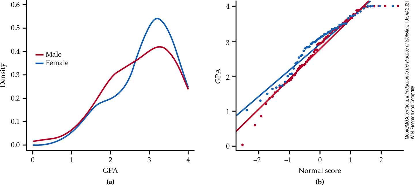
Figure 16.12 Density curves and Normal quantile plots of the distributions of GPA for males and females, Example 16.8.
Let’s consider estimating the difference between the population means,
To compute this distribution and the bootstrap standard error for the difference in sample means
Example 16.9 Assessing the bootstrap distribution.
The boot function in R automates this bootstrap procedure. Here is the R output for one set of 3000 differences:
STRATIFIED BOOTSTRAPCall:
boot(data = gpa, statistic = meanDiff, R = 3000, strata = Sex)Bootstrap Statistics : original bias std. error
t1* −0.1490259 0.003989901 0.1327419
Figure 16.13 shows that the bootstrap distribution is close to Normal. We can trust the bootstrap t confidence interval for these data. A 95% confidence interval for the difference in mean GPAs (males versus females) is, therefore,
Because Table D does not have entries for = T.INV.2T(0.05,58) to get
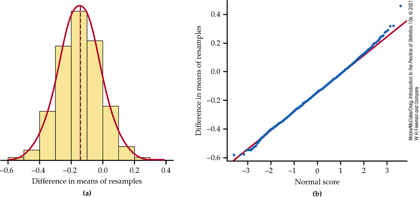
Figure 16.13 The bootstrap distribution and Normal quantile plot for the differences in means for the GPA data, Example 16.9.
We are 95% confident that the difference in the mean GPAs of males and females at this large university after three semesters is between
In this example, the bootstrap distribution of the difference is close to Normal. ![]() When the bootstrap distribution is non-Normal, we can’t trust the bootstrap t confidence interval. Fortunately, there are more general ways of using the bootstrap to get confidence intervals that can be safely applied when the bootstrap distribution is not Normal. These methods, which we discuss in Section 16.4, are the next step in practical use of the bootstrap.
When the bootstrap distribution is non-Normal, we can’t trust the bootstrap t confidence interval. Fortunately, there are more general ways of using the bootstrap to get confidence intervals that can be safely applied when the bootstrap distribution is not Normal. These methods, which we discuss in Section 16.4, are the next step in practical use of the bootstrap.
Check-in
16.5 Bootstrap comparison of average reading abilities. Table 7.4 (page 414) gives the scores on a test of reading ability for two groups of third-grade students. The treatment group used “directed reading activities,” and the control group followed the same curriculum without the activities.

Bootstrap the difference in means
Inspect the bootstrap distribution. Are the conditions met for the use of a bootstrap t confidence interval? If so, give a 95% confidence interval.
Compare the bootstrap results with the two-sample t confidence interval reported in Example 7.15 on page 415.
16.6 Formula-based versus bootstrap standard error. We have a formula (page 413) for the standard error of

Example 16.10 Do all daily numbers have an equal payoff?

The New Jersey Pick-It Lottery is a daily numbers game run by the state of New Jersey. We’ll analyze the first 254 drawings after the lottery was started in 1975.5 Buying a ticket entitles a player to pick a number between 000 and 999. Half the money bet each day goes into the prize pool. (The state takes the other half.) The state picks a winning number at random, and the prize pool is shared equally among all winning tickets.
Although all numbers are equally likely to win, numbers chosen by fewer people have bigger payoffs if they win because the prize is shared among fewer tickets. Figure 16.14 is a scatterplot of the first 254 winning numbers and their payoffs. What patterns can we see?
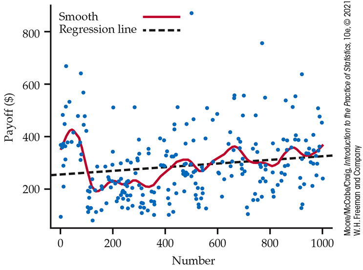
Figure 16.14 The first 254 winning numbers in the New Jersey Pick-It Lottery and the payoffs for each, Example 16.10. To see patterns, we use least-squares regression (dashed line) and a scatterplot smoother (curve).
The straight line in Figure 16.14 is the least-squares regression line. The line shows a general trend of higher payoffs for larger winning numbers. The curve in the figure was fitted to the plot by a scatterplot smoother that follows local patterns in the data rather than being constrained to a straight line. The curve suggests that there were larger payoffs for numbers in the intervals 000 to 100, 400 to 500, 600 to 700, and 800 to 999.
Are the patterns displayed by the scatterplot smoother just chance? We can use the bootstrap distribution of the smoother’s curve to get an idea of how much random variability there is in the curve. Each resample “statistic” is now a curve rather than a single number. Figure 16.15 shows the curves that result from applying the smoother to 20 resamples from the 254 data points in Figure 16.14. In practice, we’d consider many more than 20 resamples but the small number makes it easier to see the variation in resamples. The original curve is the thick line. The spread of the resample curves about the original curve shows the sampling variability of the output of the scatterplot smoother.
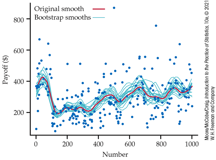
Figure 16.15 The curves produced by the scatterplot smoother for 20 resamples from the data displayed in Figure 16.14. The curve for the original sample is the heavy line.
Nearly all the bootstrap curves mimic the general pattern of the original smoother curve, showing, for example, the same low average payoffs for numbers in the 200s and 300s. This suggests that these patterns are real, not just chance. In fact, when people pick “random” numbers, they tend to choose numbers starting with 2, 3, 5, or 7, so these numbers have lower payoffs. This pattern disappeared after 1976; it appears that players noticed the pattern and changed their number choices.
Section 16.2 SUMMARY
Bootstrap distributions mimic the shape, spread, and bias of sampling distributions.
The bootstrap estimate of the bias of a statistic is the mean of the bootstrap distribution minus the statistic for the original data. Small bias means that the bootstrap distribution is centered at the statistic of the original sample and suggests that the sampling distribution of the statistic is centered at the population parameter.
The bootstrap can estimate the sampling distribution, bias, and standard error of a wide variety of statistics, such as the trimmed mean, whether or not statistical theory tells us about their sampling distributions.
If the bootstrap distribution is approximately Normal and the bias is small, we can give a bootstrap t confidence interval for the parameter
where t* is the critical value of the
To use the bootstrap to compare two populations, draw separate resamples from each sample and compute a statistic that compares the two groups. Repeat many times and use the bootstrap distribution for inference.
Section 16.2 EXERCISES
16.16 Use the bootstrap standard error and the t distribution for the confidence interval. Suppose you collect GPA data similar to that of Example 16.5 (page 16-12) from your university. You only collect
What is the bootstrap estimate of bias?
Do you think it reasonable to use the bootstrap t confidence interval? Explain your answer.
Use the t distribution to find the 95% confidence interval.
16.17 Should you use the bootstrap t confidence interval? For each of the following situations, explain whether or not you would use the bootstrap standard error and the t distribution for the confidence interval. Give reasons for your answers.
The bootstrap distribution of the mean is approximately Normal, and the difference between the mean of the data and the mean of the bootstrap distribution is large relative to the mean of the data.
The bootstrap distribution of the mean is approximately Normal, and the difference between the mean of the data and the mean of the bootstrap distribution is small relative to the mean of the data.
The bootstrap distribution of the mean is clearly skewed, and the difference between the mean of the data and the mean of the bootstrap distribution is large relative to the mean of the data.
The bootstrap distribution of the mean is clearly skewed, and the difference between the mean of the data and the mean of the bootstrap distribution is small relative to the mean of the data.
16.18 Using the mean instead of the trimmed mean. In Example 16.7 (page 16-15), bootstrap results for the 25% trimmed mean of GPA were presented. Here are some results using the mean as the statistic:
ORDINARY NONPARAMETRIC BOOTSTRAPCall:
boot(data = GPA, statistic = theta, R = 3000)Bootstrap Statistics :original bias std. error
t1* 2.842133 −0.002608911 0.06722723The bootstrap distribution (not shown) looks very Normal. Is it reasonable to construct the t confidence interval? Explain your answer.
Construct the t confidence interval.
A friend is confused about why the two analyses do not provide similar bootstrap means, especially given that both sampling distributions appear to be Normal. How would you explain this to your friend?
16.19 Bootstrap t confidence interval for the time to start a business. In Exercise 16.9 (page 16-17), we examined the bootstrap distribution for the times to start a business. Return to or re-create the bootstrap distribution of the sample mean for these 187 observations.

Find the bootstrap t 95% confidence interval for these data.
Compare the interval you found in part (a) with the usual t interval.
Which interval do you prefer? Give reasons for your answer.
16.20 Bootstrap t confidence interval for average delivery time by a robot. Return to or re-create the bootstrap distribution of the sample mean for the eight lunch delivery times in Exercise 16.11 (page 16-11).

Although the sample is small, verify using graphs and numerical summaries of the bootstrap distribution that the distribution is reasonably Normal and that the bias is small relative to the observed
The bootstrap t confidence interval for the population mean
Give the usual t 95% interval and compare it with your interval from part (b).
16.21 Bootstrap t confidence interval for help room visit lengths. Return to or re-create the bootstrap distribution of the sample mean for the 50 visit lengths in Exercise 16.14 (page 16-11).

What is the bootstrap estimate of the bias? Verify from the graphs of the bootstrap distribution that the distribution is reasonably Normal and that the bias is small relative to the observed
Give the 95% bootstrap t confidence interval for
The only difference between the bootstrap t and usual one-sample t confidence intervals is that the bootstrap interval uses
16.22 Another bootstrap distribution of the trimmed mean. Bootstrap distributions and quantities based on them differ randomly when we repeat the resampling process. A key fact is that they do not differ very much if we use a large number of resamples. Figure 16.11 (page 16-14) shows one bootstrap distribution of the trimmed mean of the GPA data. Repeat the resampling of these data to get another bootstrap distribution of the trimmed mean.
Plot the bootstrap distribution and compare it with Figure 16.11. Are the two bootstrap distributions similar?
What are the values of the bias and bootstrap standard error for your new bootstrap distribution? How do they compare with the values given on page 16-14?
Find the 95% bootstrap t confidence interval based on your bootstrap distribution. Compare it with the result in Example 16.7 (page 16-15).
16.23 Bootstrap distribution of the standard deviation s. For Example 16.5 (page 16-12), we bootstrapped the 25% trimmed mean of 150 GPAs. Another statistic whose sampling distribution is unfamiliar to us is the standard deviation s. Bootstrap s for these data. Discuss the shape and bias of the bootstrap distribution. Is the bootstrap t confidence interval for the population standard deviation
16.24 Bootstrap comparison of tree diameters. In Exercise 7.57 (page 432), you were asked to compare the mean diameter at breast height (DBH) for trees from the northern and southern halves of a land tract using a random sample of 30 trees from each region.

Use a back-to-back stemplot or side-by-side boxplots to examine the data graphically. Does it appear reasonable to use standard t procedures?
Bootstrap the difference in means
Report the bootstrap standard error and the 95% bootstrap t confidence interval.
Compare the bootstrap results with the usual two-sample t confidence interval.
16.25 Bootstrapping a Normal data set. The following data are “really Normal.” They are an SRS from the standard Normal distribution N(0, 1), produced by a software Normal random number generator.

0.01 0.34 1.21 0.58 0.92 0.90 0.11 0.23 2.40 0.08 0.75 2.29 1.23 1.56 0.42 0.56 2.69 1.09 0.10 0.30 1.47 0.45 0.41 0.54 0.08 0.32 0.34 0.51 2.47 2.99 1.27 1.55 0.80 0.89 1.27 0.56 0.25 0.29 0.99 0.10 0.30 0.05 1.44 0.91 0.51 0.48 0.02 Make a histogram and Normal quantile plot. Do the data appear to be “really Normal”? From the histogram, does the N(0, 1) distribution appear to describe the data well? Why?
Bootstrap the mean. Why do your bootstrap results suggest that t confidence intervals are appropriate?
Give both the bootstrap and the formula-based standard errors for
16.26 Bootstrap distribution of the median. We will see in Section 16.3 that bootstrap methods often work poorly for the median. To illustrate this, bootstrap the sample median of the 21 viewing times we studied in Example 16.1 (page 16-3). Why is the bootstrap t confidence interval not justified?

16.27 Bootstrap distribution of the mpg standard deviation. The Environmental Protection Agency (EPA) establishes the tests to determine the fuel economy of new cars, but it often does not perform them. Instead, the test protocols are given to the car companies, and the companies perform the tests themselves. To keep the industry honest, the EPA runs some audits each year. The following data are from one EPA audit. We studied these data in Exercise 7.11 (page 406), using methods based on Normal distributions.

18.0 15.7 15.8 18.0 18.5 19.8 20.2 20.4 16.9 18.3 19.8 17.2 16.7 17.7 19.5 18.0 In addition to the average mpg, the EPA is also interested in how much variability there is in the mpg.
Calculate the sample standard deviation s for these mpg values.
We have no formula for the standard error of s. Find the bootstrap standard error for s.
What does the standard error indicate about how accurate the sample standard deviation is as an estimate of the population standard deviation?
Would it be appropriate to give a bootstrap t interval for the population standard deviation? Why or why not?