16.4 Bootstrap Confidence Intervals
Until now, we have met just one type of inference procedure based on resampling: the bootstrap t confidence intervals. We can calculate a bootstrap t confidence interval for any parameter by bootstrapping the corresponding statistic. We don’t need conditions on the population or special knowledge about the sampling distribution of the statistic.
The flexible and almost automatic nature of bootstrap t intervals is appealing—but there is a catch. These intervals work well only when the bootstrap distribution tells us that the sampling distribution is approximately Normal and has small bias. How well must these conditions be met? What can we do if we don’t trust the bootstrap t interval? In this section, we will see how to quickly check t confidence intervals for accuracy, and we will learn alternative bootstrap confidence intervals that can be used more generally.
Bootstrap percentile confidence intervals
Confidence intervals are based on the sampling distribution of a statistic. If a statistic has no bias as an estimator of a parameter, its sampling distribution is centered at the true value of the parameter. We can then get a 95% confidence interval by marking off the central 95% of the sampling distribution. The t critical values in a t confidence interval are a shortcut to marking off the central 95%.
This shortcut doesn’t work under all conditions—it depends both on lack of bias and on Normality. One way to check whether t intervals (using either bootstrap or formula-based standard errors) are reasonable is to compare them with the central 95% of the bootstrap distribution. The 2.5 and 97.5 percentiles mark off the central 95%. The interval between the 2.5 and 97.5 percentiles of the bootstrap distribution is often used as a confidence interval in its own right. It is known as a bootstrap percentile confidence interval. This is the interval we used when we introduced the bootstrap (page 403) in Chapter 7.
The advantages of bootstrap percentile intervals over bootstrap t intervals is that they do not ignore skewness. Percentile intervals are therefore usually more accurate, as long as the estimate of bias is small.
![]() Because we will soon meet a much more accurate bootstrap interval
that handles both bias and skewness, we only reccomend the bootstrap
percentile interval when it is reasonably similar to bootstrap t
interval.
This will occur when the estimate of bias is small and the skewness is
relatively mild.
Because we will soon meet a much more accurate bootstrap interval
that handles both bias and skewness, we only reccomend the bootstrap
percentile interval when it is reasonably similar to bootstrap t
interval.
This will occur when the estimate of bias is small and the skewness is
relatively mild.
Example 16.11 Bootstrap percentile confidence interval for the trimmed mean.
In Example 16.7 (page 16-15), we found that a 95% bootstrap t confidence interval for the 25% trimmed mean of GPA for the population of college students after three semesters at this large university is between 2.795 and 3.105. The bootstrap distribution in Figure 16.11 shows a small bias and, though close to Normal, is a bit skewed. Is the bootstrap t confidence interval accurate for these data?
We can use the quantile function in R to compute the needed percentiles of our 3000 resamples. For this bootstrap distribution, the 2.5 and 97.5 percentiles are 2.793 and 3.095, respectively. These are the endpoints of the 95% bootstrap percentile confidence interval. This interval is quite close to the bootstrap t interval. We conclude that the bootstrap t interval is reasonably accurate.
The bootstrap t interval for the trimmed mean of GPA in Example 16.7 is
We can learn something by also writing the percentile interval
starting at the statistic
Unlike the t interval, the percentile interval is not symmetric—its endpoints are different distances from the statistic. The slightly greater distance to the 2.5 percentile reflects the slight left-skewness of the bootstrap distribution. Given that the bias is small, we’d expect this interval to be slightly more accurate than the equitailed bootstrap t interval.
Check-in
-
16.7 Determining the percentile endpoints. What percentiles of the bootstrap distribution are the endpoints of a 99% bootstrap percentile confidence interval? How do they change for a 90% bootstrap percentile confidence interval?
-
16.8 Bootstrap percentile confidence interval for profile viewing time. Consider the small sample of Facebook viewing times in Check-in question 16.1 (page 16-6). Bootstrap the sample mean using 2000 resamples.

-
Make a histogram and a Normal quantile plot of these 2000 sample means. Does the bootstrap distribution appear close to Normal? Is the bias small relative to the observed sample mean?
-
Find the 95% bootstrap t confidence interval.
-
Give the 95% confidence percentile interval and compare it with the interval in part (b).
-
Should we use one of these intervals? Explain your reasoning.
-
A more accurate bootstrap confidence interval: BCa
Any method for obtaining confidence intervals requires some conditions in order to produce exactly the intended confidence level. These conditions (for example, Normality) are never exactly met in practice. So a 95% confidence interval in practice will not capture the true parameter value exactly 95% of the time.
In addition to “hitting” the parameter 95% of the time, a good confidence interval should divide its 5% of “misses” equally between high misses and low misses. We will say that a method for obtaining 95% confidence intervals is accurate in a particular setting if 95% of the time it produces intervals that capture the parameter and if the 5% of misses are equally shared between high and low misses. Perfect accuracy isn’t available in practice, but some methods are more accurate than others.
One advantage of the bootstrap is that we can to some extent check the accuracy of the bootstrap t and percentile confidence intervals by examining the bootstrap distribution for bias and skewness and by comparing the two intervals with each other. The interval in Example 16.11 reveals a slight left-skewness that does little to alter our inference.
![]() In general, the t and percentile intervals may not be sufficiently
accurate when
In general, the t and percentile intervals may not be sufficiently
accurate when
- The statistic is strongly biased, as indicated by the bootstrap estimate of bias.
- The sampling distribution of the statistic is clearly skewed, as indicated by the bootstrap distribution and by comparing the t and percentile intervals.
Most confidence interval procedures are more accurate for larger
sample sizes. The accuracies of the t and percentile procedures
improve only slowly: they require 100 times more data to improve
accuracy by a factor of 10. (Recall the
This method is accurate in a wide variety of settings, has reasonable computation requirements (by modern standards), and does not produce excessively wide intervals. The BCa intervals are among the most widely used intervals. Because the BCa method is related to the percentile method, it is still based on the key ideas of resampling and the bootstrap distribution.
You should always use this more accurate method (or an alternative,
such as tilting intervals) if your software offers it. The details of
producing confidence intervals are quite technical.6
The BCa method requires more than 1000 resamples for high accuracy. We
recommend that you use 5000 or more resamples.
![]() Don’t forget that even BCa confidence intervals should be used
cautiously when sample sizes are small because there are not enough
data to accurately determine the necessary corrections for bias and
skewness.
Don’t forget that even BCa confidence intervals should be used
cautiously when sample sizes are small because there are not enough
data to accurately determine the necessary corrections for bias and
skewness.
Example 16.12 The BCa confidence interval for the ratio of variances.
![]()
In Example 16.9 (page 16-17), we compared the GPA means of men and women using a 95% bootstrap t confidence interval. Because 0 was contained in the interval, we concluded that there was not enough evidence to state that the two means were different. Suppose we also want to compare the variances. The densities in Figure 16.12 (page 16-17) suggest that the spread among the male GPAs is larger than that of the females. The ratio of the male sample variance to the female sample variance is 1.321. Can we conclude there is a difference?
In
Section 12.1
(page 599), we
discussed the modified Levene’s test for equality of spread. Let’s
now instead use the bootstrap to test equality. Specifically, we’ll
form a 95% confidence interval for
Figure 16.19
shows the bootstrap distribution of the ratio of sample variances
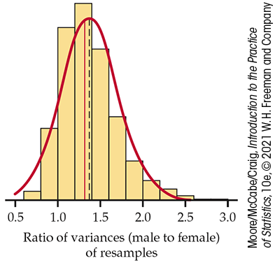
Figure 16.19 The bootstrap distribution of the ratio of sample variances of 5000 resamples from the data in Example 16.8. The bootstrap distribution is right-skewed, so we conclude that the sampling distribution of the ratio of sample variances is right-skewed, Example 16.12.
The bootstrap t and percentile intervals aren’t reliable when the sampling distribution of the statistic is strongly skewed. Figure 16.20 shows software output that includes the percentile and BCa intervals. The bootstrap t interval is closely related to the Normal interval that is also supplied. The basic confidence interval is another method based on the percentiles of the bootstrap distribution that we will not discuss here.
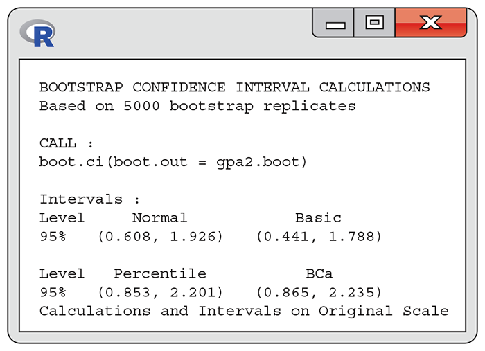
Figure 16.20 R output for bootstrapping the ratio of variances for the GPA data, Example 16.12.
The BCa interval is
and the percentile interval is
In this case, the percentile and BCa intervals are similar, but the BCa is shifted slightly as it has adjusted for the bias, which was estimated at 0.054. Both intervals are strongly asymmetrical: the upper endpoint is about twice as far from the sample ratio as the lower endpoint. This reflects the strong right-skewness of the bootstrap distribution.
The output in Figure 16.20 also shows that both endpoints of the less- accurate intervals (bootstrap t via the Normal interval and the percentile interval) are too low. These intervals miss the population ratio on the low side too often (more than 2.5% of the time) and miss on the high side too seldom. They give a biased picture of where the true ratio is likely to be.
Confidence intervals for the correlation
The bootstrap allows us to find confidence intervals for a wide variety of statistics. So far, we have looked at the sample mean and trimmed mean, the difference between two means, and the ratio of sample variances using a variety of different bootstrap confidence intervals. The choice of interval depended on the shape of the bootstrap distribution and the desired accuracy.
Now we will bootstrap the correlation coefficient. This is our first use of the bootstrap for a statistic that depends on two related variables. As with the difference between two means, we must pay attention to how we should resample.
Example 16.13 Correlation between price and rating.
![]()

An article in Consumer Reports rated laundry detergents on a scale from 1 to 100.7 Here are the ratings, along with the price per load, in cents, for 24 laundry detergents:
| Rating | Price (cents) | Rating | Price (cents) | Rating | Price (cents) | Rating | Price (cents) |
|---|---|---|---|---|---|---|---|
| 61 | 17 | 59 | 22 | 56 | 22 | 55 | 16 |
| 55 | 30 | 52 | 23 | 51 | 11 | 50 | 15 |
| 50 | 9 | 48 | 16 | 48 | 15 | 48 | 18 |
| 46 | 13 | 46 | 13 | 45 | 17 | 36 | 8 |
| 35 | 8 | 34 | 12 | 33 | 7 | 32 | 6 |
| 32 | 5 | 29 | 14 | 26 | 11 | 26 | 13 |
In Example 2.9 (page 77), we examined the relationship between rating and price per load for 53 laundry detergents. Based on that analysis, we expect that the higher-priced detergents will tend to have higher ratings. The scatterplot in Figure 16.21 shows that for these data, the higher-priced products do tend to have better ratings. In fact, the relationship appears to be stronger than what we observed in Chapter 2. The correlation is 0.671. Let’s use the bootstrap to find a 95% confidence interval for the population correlation.
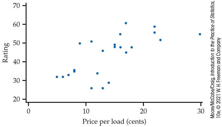
Figure 16.21Scatterplot of price per load (in cents) versus rating for 24 laundry detergents, Example 16.13.
Our confidence interval will also provide a test of the null
hypothesis that the population correlation is zero. If the 95%
confidence interval does not include zero, we can reject the null
hypothesis in favor of the two-sided alternative. Although we would
expect the correlation to be positive, we could be surprised and find
that it is negative. It is important to keep in mind that
![]() we cannot use what we learned by looking at the scatterplot to
formulate our alternative hypothesis.
we cannot use what we learned by looking at the scatterplot to
formulate our alternative hypothesis.
How shall we resample from the laundry detergent data? Because each observation consists of the price and the rating for one product, we resample products. Resampling prices and ratings separately would cause us to lose the connection between a product’s price and its rating. Software such as R automates proper resampling. Once we have produced a bootstrap distribution by resampling, we can examine the distribution and construct a confidence interval in the usual way. We need no special formulas or procedures to handle the correlation.
Example 16.14 Reporting the bootstrap results.
Figure 16.22 shows the bootstrap distribution and Normal quantile plot for the sample correlation for 5000 resamples from the 24 laundry detergents in our sample. The bootstrap distribution is skewed to the left, with relatively small bias. We need to check whether a 95% bootstrap percentile confidence interval is reasonable here.
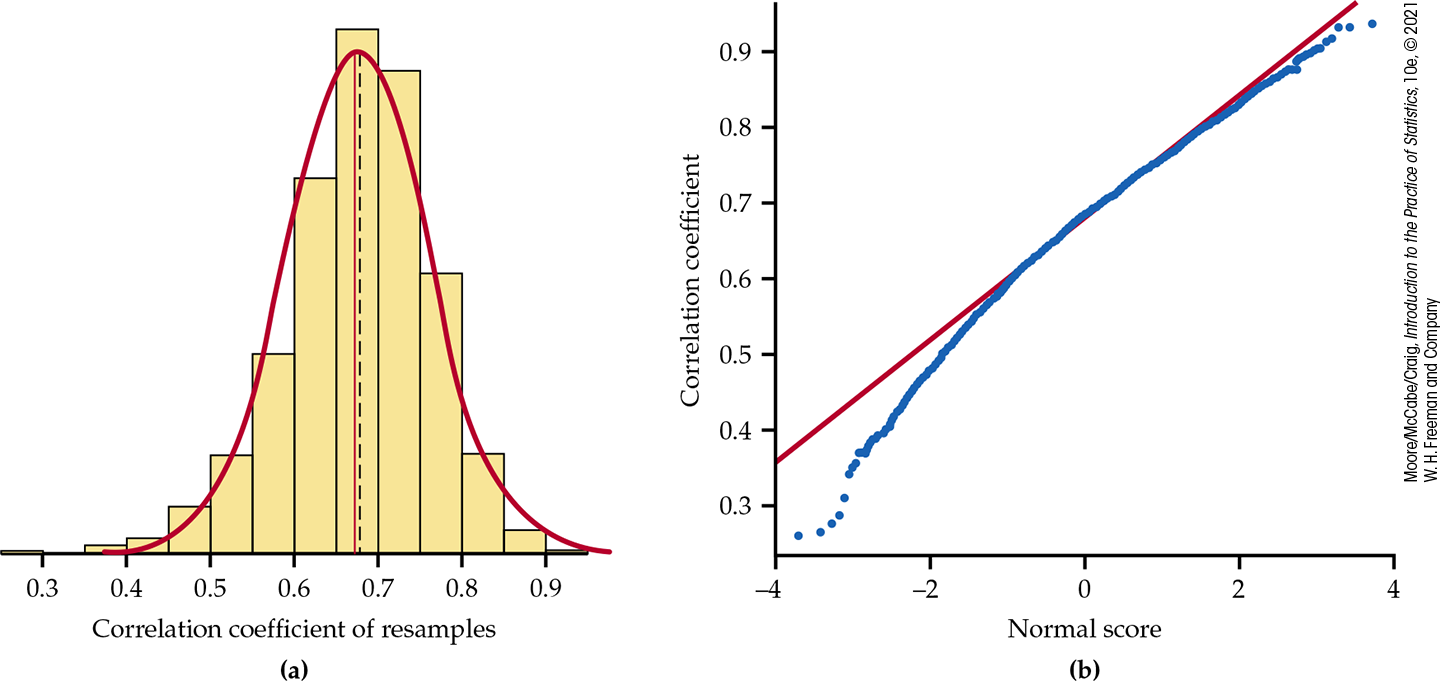
Figure 16.22 The bootstrap distribution and Normal quantile plot for the correlation r for 5000 resamples from the laundry detergent data set, Example 16.14.
The bootstrap standard error is
The 95% bootstrap percentile interval is
The two confidence intervals are not too different. However, given the skewness of the sampling distribution, the BCa interval is the better choice
This interval is shifted more to the left and is more asymmetric.
While the confidence intervals give a wide range for the population correlation, both of them include only positive values. Thus, these data provide significant evidence that there is a positive relationship between a laundry detergent’s rating and its price per load.
Section 16.4 SUMMARY
- Both bootstrap t and (when they exist) traditional z and t confidence intervals require statistics with small bias and sampling distributions close to Normal. We can check these conditions by examining the bootstrap distribution for bias and lack of Normality.
- The bootstrap percentile confidence interval for 95% confidence is the interval from the 2.5 percentile to the 97.5 percentile of the bootstrap distribution. Agreement between the bootstrap t and percentile intervals is an added check on the conditions needed by the t interval. Do not use t or percentile intervals if these conditions are not met.
- When bias or skewness is present in the bootstrap distribution, use a BCa interval. The t and percentile intervals are inaccurate under these circumstances unless the sample sizes are very large. The BCa confidence intervals adjust for bias and skewness and are generally accurate except for small samples.
Section 16.4 EXERCISES
-
16.32 Find the 95% bootstrap percentile confidence interval. A farmer is interested in the average weight of his pigs at six months of age. The mean of a sample of
Percentile 0.01 0.025 0.05 0.10 0.50 0.90 0.95 0.975 0.99 216.9 218.2 219.3 220.5 225.0 229.3 230.7 231.6 233.0 -
Find both the 95% bootstrap t and 95% bootstrap percentile confidence intervals.
Which of these intervals do you prefer, and why?
-
-
16.33 Summarize the output. Figures 16.23 and 16.24 show R output regarding a comparison of two variances with samples
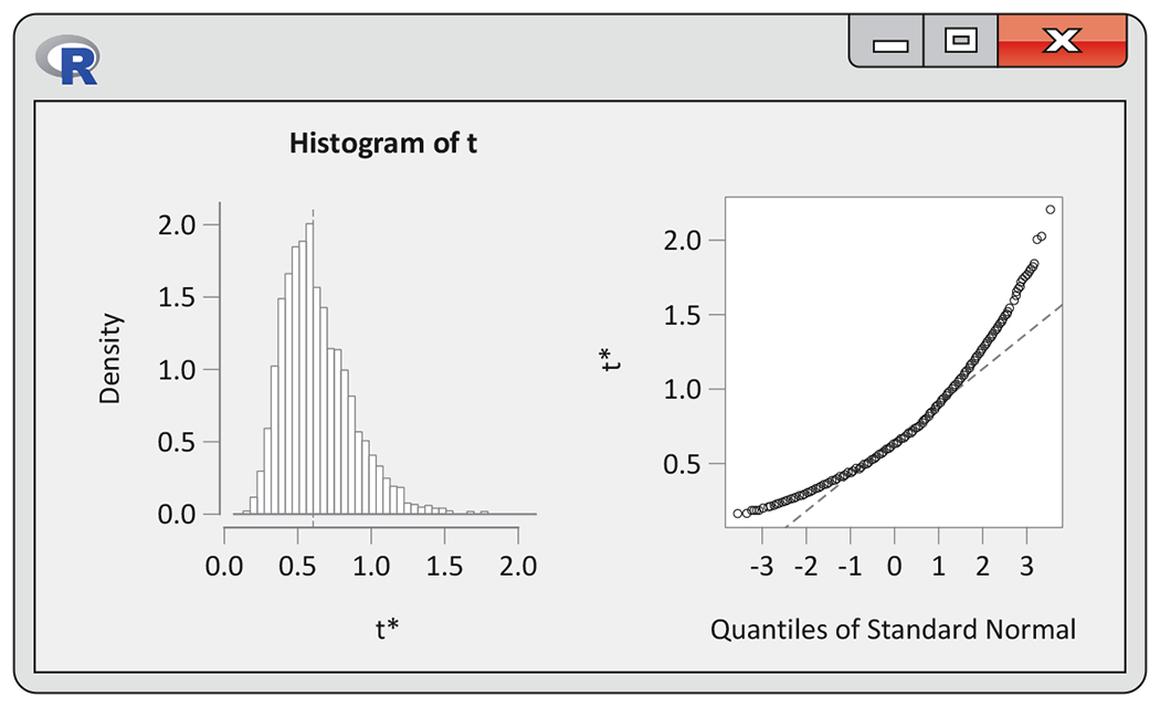
Figure 16.23 R graphical output, Exercise 16.33.
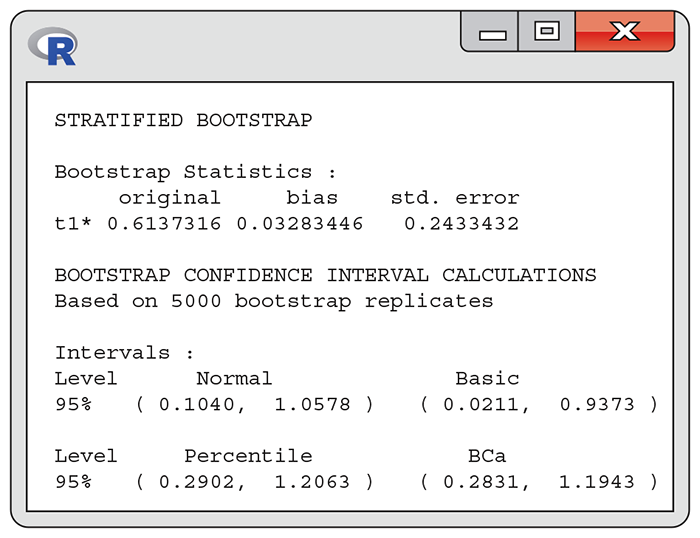
Figure 16.24 R bootstrap and confidence interval output, Exercise 16.33.
-
16.34 Confidence interval for the average IQ score. The distribution of the 60 IQ test scores in Table 1.1 (page 15) is roughly Normal, and the sample size is large enough that we expect a Normal sampling distribution. We will compare confidence intervals for the population mean IQ

-
Use the formula
-
Bootstrap the mean of the IQ scores. Make a histogram and a Normal quantile plot of the bootstrap distribution. Does the bootstrap distribution appear to be Normal? What is the bootstrap standard error? Give the 95% bootstrap t confidence interval.
-
Give the 95% confidence percentile and BCa intervals. Make a graphical comparison by drawing a vertical line at the original sample mean
-
-
16.35 Confidence interval for a Normal data set. In Exercise 16.25 (page 16-22), you bootstrapped the mean of a simulated SRS from the standard Normal distribution N(0, 1) and found the 95% standard t and bootstrap t confidence intervals for the mean.

-
Find the 95% bootstrap percentile confidence interval. Does this interval confirm that the t intervals are acceptable?
-
We know that the population mean is 0. Do the confidence intervals capture this mean?
-
-
16.36 Using bootstrapping to check traditional methods. Bootstrapping is a good way to check whether traditional inference methods are accurate for a given sample. Consider the following data:

98 107 113 104 94 100 107 98 112 97 99 95 97 90 109 102 89 101 93 95 95 87 91 101 119 116 91 95 95 104 -
Examine the data graphically. Do they appear to violate any of the conditions needed to use the one-sample t confidence interval for the population mean?
-
Calculate the 95% one-sample t confidence interval for this sample.
-
Bootstrap the data and inspect the bootstrap distribution of the mean. Does it suggest that a t interval should be reasonably accurate? Calculate the bootstrap t 95% interval.
-
Find the 95% bootstrap percentile interval. Does it agree with the two t intervals? What do you conclude about the accuracy of the one-sample t interval here?
-
-
16.37 Comparing bootstrap confidence intervals. Although the graphs in Figure 16.13 (page 16-18) do not appear to show any important skewness in the bootstrap distribution of the difference in means for Example 16.9, there is evidence that the right tail is slightly longer than expected. Using the Example 16.11 (page 16-29) comparison of the bootstrap percentile and bootstrap t intervals as a guide, describe what you might expect to see if you computed the bootstrap percentile confidence interval for the data in Example 16.9.
-
16.38 More on using bootstrapping to check traditional methods. Continue to work with the data given in Exercise 16.36.
Find the 95% BCa confidence interval.
-
Does your opinion of the robustness of the one-sample t confidence interval change when you compare it with the BCa interval?
-
To check the accuracy of the one-sample t confidence interval, would you generally use the bootstrap percentile or the BCa interval? Explain.
-
16.39 BCa interval for the correlation coefficient. Find the 95% BCa confidence interval for the correlation between price and rating, from the data in Example 16.13 (page 16-33). Is this more accurate interval in general agreement with the 95% bootstrap t and percentile intervals? Do you still agree with the judgment in the discussion of Example 16.14 that the simpler intervals are adequate?

-
16.40 Bootstrap confidence intervals for the average audio file length. In Check-in question 16.4 (page 16-16), you found a bootstrap t confidence interval for the population mean

-
16.41 Bootstrap confidence intervals for visits to a help room. The distribution of the visit lengths to a statistics help room that you used in Exercise 16.21 (page 16-21) is skewed. In that exercise, you found a bootstrap t confidence interval for the population mean

-
16.42 Bootstrap confidence intervals for the standard deviation. We would like a 95% confidence interval for the standard deviation

-
16.43 The effect of decreasing the sample size. Exercise 16.15 (page 16-11) gives an SRS of 10 of the visit lengths from Table 5.1 (page 283). Describe the bootstrap distribution of

-
16.44 Bootstrap confidence interval for the GPA data. The GPA data for females from Example 16.8 (page 16-16) are strongly skewed to the left and have a cluster of observations at 4.
-
Bootstrap the mean of the data. Based on the bootstrap distribution, which bootstrap confidence intervals would you consider for use? Explain your answer.
-
Find all three bootstrap confidence intervals. How do the intervals compare? Briefly explain the reasons for any differences. In particular, what kind of errors would you make in estimating the mean GPA by using a t interval or a percentile interval instead of a BCa interval?
-
-
16.45 Bootstrap confidence intervals for the difference in GPAs. Example 16.9 (page 16-17) considers the difference in mean GPAs of men and women. The bootstrap distribution appeared reasonably Normal. Give the 95% BCa confidence interval for the difference in mean GPAs. Is this interval comparable to the bootstrap t interval calculated in the example?
-
16.46 The correlation between GPA and high school math grades. The study described in Example 16.5 (page 16-12) used high school grades to predict GPA. For this exercise, we will look at the correlation between GPA and high school math grades.
-
Describe the distribution of GPAs. Do the same for high school math grades.
-
Describe the relationship between GPA and high school math grades.
-
Generate 2000 resamples and use them to obtain the bootstrap distribution for the correlation.
-
Describe the shape and bias of the bootstrap distribution. Does use of the simpler bootstrap confidence intervals (t and percentile) appear to be justified?
-
Find all three 95% bootstrap confidence intervals: t, percentile, and BCa. Make a graphical comparison by drawing a vertical line at the original correlation r and displaying the three intervals vertically, one above the other. Discuss what you see. Does it still appear that the simpler intervals are justified? What confidence interval would you include in a report describing the relationship between GPA and high school math grades?
-
-
16.47 The correlation between BMI and physical activity. Figure 10.3 (page 518) shows a relatively weak negative relationship between BMI and physical activity. Use the bootstrap to perform statistical inference for the correlation.

-
Describe the shape and bias of the bootstrap distribution. Do you think that a simple bootstrap inference (t and percentile confidence intervals) is justified? Explain your answer.
-
Give the 95% BCa and bootstrap percentile confidence intervals for the population correlation. Do they (as expected) agree closely? Do these intervals provide significant evidence at the 5% level that the population correlation is not 0?
-
-
16.48 Bootstrap distribution for the slope
-
16.49 Predicting ratings of laundry detergents. Refer to Example 16.13 (page 16-33).
-
Find the least-squares regression line for predicting rating from price.
-
Bootstrap the regression line and give a 95% confidence interval for the slope of the population regression line.
-
Compare the bootstrap results with the usual method for finding a confidence interval for a regression slope.
-
-
16.50 Predicting GPA. Continue your study of GPA and high school math grades, begun in Exercise 16.46, by performing a regression to predict GPA using high school math grades as the explanatory variable.
-
Plot the residuals against the math grades and make a Normal quantile plot of the residuals. Do these plots suggest that inference based on the usual simple linear regression model may be inaccurate? Give reasons for your answer.
-
Bootstrap the least-squares regression line and examine the bootstrap distribution of the slope
-
Give the 95% BCa confidence interval for the slope
-
-
16.51 Predicting BMI. Continue your study of the relationship between BMI and physical activity, begun in Exercise 16.47. Bootstrap the least-squares regression line using physical activity as the explanatory variable.
-
Examine the shape and bias of the bootstrap distribution of the slope
-
Find the BCa, bootstrap t, and bootstrap percentile confidence intervals and compare them with the standard 95% t confidence interval for
-
-
16.52 The effect of outliers. We know that outliers can strongly influence statistics such as the mean and the least-squares line. A study of dementia patients in nursing homes recorded various types of disruptive behaviors every day for 12 weeks. Days were classified as moon days if they were in a three-day period centered at the day of a full moon. A matched pairs analysis was performed to see if the average number of disruptive behaviors was different on moon days. There were three patients with very small differences that may be considered outliers.

-
Bootstrap the mean of the differences between moon days and other days, with and without the three low values. How do these values influence the shape and bias of the bootstrap distribution?
-
Give the BCa confidence interval from both bootstrap distributions. Discuss the differences.
-