16.5 Significance Testing Using Permutation Tests
Significance tests tell us whether an observed effect, such as a difference between two means or a correlation between two variables, could reasonably occur “just by chance” in selecting a random sample. If not, we have evidence that the effect observed in the sample reflects an effect that is present in the population. The reasoning of tests goes like this:
- Choose a statistic that measures the effect you are looking for.
- Construct the sampling distribution that this statistic would have if the effect were not present in the population.
- Locate the observed statistic on this distribution. A value in the main body of the distribution could easily occur just by chance. A value in the tails would rarely occur by chance and so provides evidence that something other than chance is operating.
The statement that the effect we seek is not present in the
population is the null hypothesis,
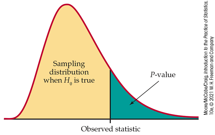
Figure 16.25 The P-value of a statistical test is found from the sampling distribution the statistic would have if the null hypothesis were true. It is the probability of a result at least as extreme as the value we actually observed.
Tests based on resampling don’t change this approach. They just find P-values by resampling calculations rather than from assumed distributions. Using resampling also means that these tests can be used in settings where traditional tests don’t apply.
Because P-values are calculated as if the null hypothesis were true, we cannot resample from the observed sample as we did earlier. In the absence of bias, resampling from the original sample creates a bootstrap distribution centered at the observed value of the statistic. If the null hypothesis is, in fact, not true, this value may be far from the parameter value stated by the null hypothesis. We must estimate what the sampling distribution of the statistic would be if the null hypothesis were true. That is, we must obey the following rule:
Example 16.15 “Directed reading activities”.
![]()
In Example 7.14 (page 414), we applied the two-sample t test to see if new “directed reading activities” improve the reading ability of elementary school students. The study assigned students at random to either the new methods (Treatment group, 21 students) or traditional teaching methods (Control group, 23 students).8 At the end of eight weeks, the Degree of Reading Power (DRP) score was obtained. These data are shown in Table 16.1.
| Treatment group | Control group | ||||||
|---|---|---|---|---|---|---|---|
| 24 | 61 | 59 | 46 | 42 | 33 | 46 | 37 |
| 43 | 44 | 52 | 43 | 43 | 41 | 10 | 42 |
| 58 | 67 | 62 | 57 | 55 | 19 | 17 | 55 |
| 71 | 49 | 54 | 26 | 54 | 60 | 28 | |
| 43 | 53 | 57 | 62 | 20 | 53 | 48 | |
| 49 | 56 | 33 | 37 | 85 | 42 | ||
Instead of the two-sample t statistic, we will use the difference between the sample means as our measure of the effect of the new activities:
The null hypothesis
Describing
Here is an outline of the permutation test procedure for comparing the mean DRP scores in Example 16.15:
-
Choose 21 of the 44 students at random to be the treatment group; the other 23 are the control group. This is an ordinary SRS, chosen without replacement. It is called a permutation resample.
-
Calculate the mean DRP score in each group, using the students’ DRP scores in Table 16.1. The difference between these means is our statistic.
-
Repeat this resampling and calculation of the statistic hundreds of times. The distribution of the statistic from these resamples estimates the sampling distribution under the condition that
-
Consider the value of the statistic actually observed in the study,
Locate this value on the permutation distribution to get the P-value.
Figure 16.26 illustrates permutation resampling on a small scale. The top box shows the results of a study with four subjects in the treatment group and two subjects in the control group. A permutation resample chooses an SRS of four of the six subjects to form the treatment group. The remaining two are the control group. The results of three permutation resamples appear below the original results, along with the statistic (difference in group means) for each.
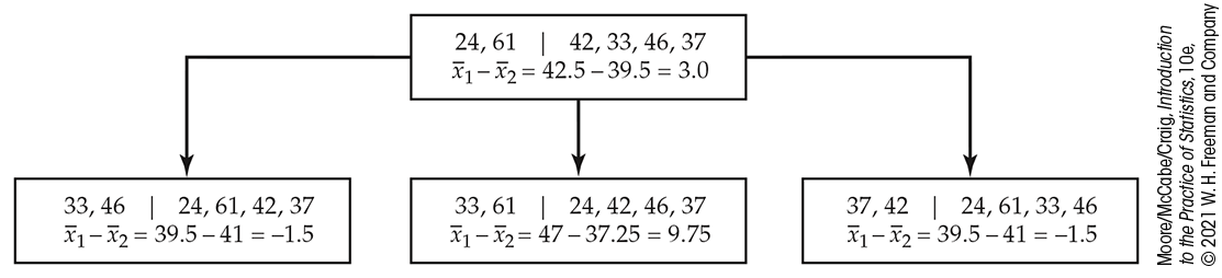
Figure 16.26 The idea of permutation resampling. The top box shows the outcome of a study with four subjects in one group and two in the other. The boxes below show three permutation resamples. The values of the statistic for many such resamples form the permutation distribution.
Example 16.16 Permutation test for the DRP study.
![]()
Figure 16.27
shows the permutation distribution of the difference in means based on
1000 permutation resamples from the DRP data in
Table 16.1. This
is a resampling estimate of the sampling distribution of the statistic
when the null hypothesis
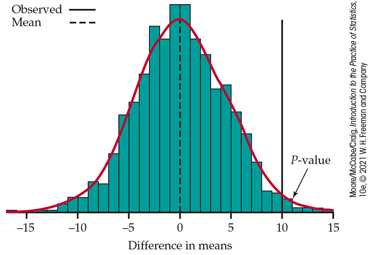
Figure 16.27 The permutation distribution of the difference between the treatment mean and the control mean based on the DRP scores of 44 students, Example 16.16. The dashed line marks the mean of the permutation distribution: it is very close to zero, the value specified by the null hypothesis. The solid vertical line marks the observed difference in means, 9.954. Its location in the right tail shows that a value this large is unlikely to occur when the null hypothesis is true.
We seek evidence that the treatment increases DRP scores, so the
alternative hypothesis is that the distribution of the statistic
Figure 16.27 shows
that the permutation distribution has a roughly Normal shape. Because
the permutation distribution approximates the sampling distribution, we
now know that the sampling distribution is close to Normal. When the
sampling distribution is close to Normal, we can safely apply the usual
two-sample t test. The JMP output in
Figure 7.15 (page 415) gives
Using software
In principle, you can program almost any statistical software to do a
permutation test. It is more convenient to use software that automates
the process of resampling, calculating the statistic, forming the
permutation distribution, and finding the P-value. The package
perm in R contains functions that allow you to request
permutation tests. The permutation distribution in
Figure 16.27 is
one output. Another is a summary of the test results:
Exact Permutation Test Estimated by Monte Carlo
data: trtgrp and ctrlgrp
p-value = 0.0154
alternative
            hypothesis: true mean trtgrp - mean ctrlgrp is greater than 0 sample
            estimates:
mean trtgrp − mean ctrlgrp
          9.954451
p-value
            estimated from 5000 Monte Carlo replications
99 percent
            confidence interval on p-value:
 0.01110640 0.02024333
By giving “greater” as the alternative hypothesis, the output makes it clear that 0.0154 is the one-sided P-value. This estimate of the P-value is more precise than the 0.014 estimate because it is based on 5000 rather than 1000 resamples.
Permutation tests in practice
We have analyzed the data in Table 16.1 both by using the two-sample t test (in Chapter 7) and by using a permutation test. Comparing the two approaches brings out some general points about permutation tests versus traditional formula-based tests.
Permutation tests versus t tests
There are several advantages of the permutation test over the two-sample t test:
-
The hypotheses for the t test are stated in terms of the two population means,
The permutation test hypotheses are more general. The null hypothesis is “same distribution of scores in both groups,” and the one-sided alternative is “scores in the treatment group are systematically larger.” These more general hypotheses imply the t hypotheses if we are interested in mean scores and the two distributions have the same shape.
-
The plug-in principle (page 16-8) says that the difference in sample means estimates the difference in population means. The t statistic starts with this difference. We used the same statistic in the permutation test, but that was a choice: we could use the difference in 25% trimmed means or any other statistic that measures the effect of treatment versus control.
-
The t test statistic is based on standardizing the difference in means in a clever way to get a statistic that has a t distribution when
-
The t test gives accurate P-values if the sampling distribution of the difference in means is at least roughly Normal. The permutation test gives accurate P-values even when the sampling distribution is not close to Normal.
The permutation test is useful even if we plan to use the two-sample t test. Rather than rely on Normal quantile plots of the two samples and the central limit theorem, we can directly check the Normality of the sampling distribution by looking at the permutation distribution. Permutation tests provide a “gold standard” for assessing two-sample t tests. If the two P-values differ considerably, it usually indicates that the conditions for the two-sample t test don’t hold for these data. Because permutation tests give accurate P-values even when the sampling distribution is skewed, they are often used when accuracy is very important. Here is an example.
Example 16.17 Permutation test for GPAs.
![]()
In Example 16.8 (page 16-16), we looked at the difference in mean GPAs of male and female students. Figure 16.12 (page 16-17) shows both distributions. Because the distributions are skewed and the sample sizes are somewhat different, a two-sample t test might be inaccurate.
Based on the summary statistics,
| Sex | n |
|
s |
|---|---|---|---|
| Male | 91 | 2.784 | 0.859 |
| Female | 59 | 2.933 | 0.748 |
| Difference |
|
the t statistic is
We perform permutation tests with 5000 resamples using R. We use
the difference in means,
A 99% confidence interval for the P-value based on the 5000 resamples is (0.256, 0.309). This interval contains the P-value for the t test. The skewness and differing sample sizes do not have an impact here primarily because the sample sizes are relatively large.
Permutation tests versus Wilcoxon rank sum tests
The Wilcoxon rank sum test of
Chapter 15 is also
nonparametric and shares the same null hypothesis as the permutation
test. Calculation of the sampling distribution under
Data from an entire population
A subtle difference between confidence intervals and significance tests is that confidence intervals require the distinction between sample and population, but tests do not. If we have data on an entire population—say, all employees of a large corporation—we don’t need a confidence interval to estimate the difference between the mean salaries of male and female employees. We can calculate the means for all men and for all women and get an exact answer. But it still makes sense to ask, “Is the difference in means so large that it would rarely occur just by chance?” A test and its P-value answer this question.
Permutation tests provide a convenient way to answer such questions. In carrying out such a test, we pay no attention to whether the data are a sample or an entire population. The resampling assigns the full set of observed salaries at random to men and women and builds a permutation distribution from repeated random assignments. We can then see if the observed difference in mean salaries is so large that it would rarely occur if sex did not matter.
When are permutation tests valid?
The two-sample t test starts from the condition that the
sampling distribution of
![]() resampling in a way that moves observations between the two
groups requires that the two populations be identical when the
null hypothesis is true—that not only their means are the same but
also their spreads and shapes.
Our preferred version of the two-sample t allows different
standard deviations in the two groups, so the shapes are both Normal
but need not have the same spread.
resampling in a way that moves observations between the two
groups requires that the two populations be identical when the
null hypothesis is true—that not only their means are the same but
also their spreads and shapes.
Our preferred version of the two-sample t allows different
standard deviations in the two groups, so the shapes are both Normal
but need not have the same spread.
In Example 16.17, the distributions are skewed, but we do not rule out the t test because of the central limit theorem. The permutation test is valid if the GPA distributions for males and females have the same shape, so that they are identical under the null hypothesis that the centers (the means) are the same. Based on Figure 16.12 (page 16-17), it appears that the distribution for the males has a little more spread than the distribution for the females. Fortunately, the permutation test is robust. That is, it gives accurate P-values when the two population distributions have somewhat different shapes, such as when they have slightly different standard deviations.
Sources of variation
Just as in the case of bootstrap confidence intervals, permutation tests are subject to two sources of random variability: the original sample is chosen at random from the population, and the resamples are chosen at random from the sample. Again, as in the case of the bootstrap, the added variation due to resampling is usually small, and we can make it as small as we like by increasing the number of resamples.
The number of resamples on which a permutation test is based
determines the number of decimal places and precision in the
resulting P-value. Tests based on 1000 resamples give
P-values to three places (multiples of 0.001), with a margin
of error of
Check-in
-
16.9 Is a permutation test valid? Suppose a professor wants to compare the effectiveness of two different instruction methods. By design, one method is more team oriented, so he expects the variability in individual tests scores for this method to be smaller. Is it valid to use a permutation test to compare the mean scores of the two methods? Explain.
-
16.10 Declaring significance. Suppose that a one-sided permutation test based on 250 permutation resamples resulted in a P-value of 0.044. What is the approximate standard deviation of the distribution? Would you feel comfortable declaring the results significant at the 5% level? Explain.
Permutation tests in other settings
The bootstrap procedure can replace many different formula-based confidence intervals, provided that we resample in a way that matches the setting. Permutation testing is also a general method that we can adapt to various settings.
Permutation test for matched pairs.
The key step in the general procedure for permutation tests is to form permutation resamples in a way that is consistent with the study design and with the null hypothesis. Our examples to this point have concerned two-sample settings. How must we modify our procedure for a matched pairs design?
Example 16.18 Permutation test for full-moon study.
![]()

Can the full moon influence behavior? A study observed 15
nursing-home patients with dementia. The number of incidents of
aggressive behavior was recorded each day for 12 weeks. Call a day
a “moon day” if it is the day of a full moon or the day before or
after a full moon.
Table 16.2
gives the average number of aggressive incidents for moon days and
other days for each subject.9
These are matched pairs data. A matched pairs t test found
evidence that the mean number of aggressive incidents is higher on
moon days
| Patient | Moon days | Other days | Patient | Moon days | Other days |
|---|---|---|---|---|---|
| 1 | 3.33 | 0.27 | 9 | 6.00 | 1.59 |
| 2 | 3.67 | 0.59 | 10 | 4.33 | 0.60 |
| 3 | 2.67 | 0.32 | 11 | 3.33 | 0.65 |
| 4 | 3.33 | 0.19 | 12 | 0.67 | 0.69 |
| 5 | 3.33 | 1.26 | 13 | 1.33 | 1.26 |
| 6 | 3.67 | 0.11 | 14 | 0.33 | 0.23 |
| 7 | 4.67 | 0.30 | 15 | 2.00 | 0.38 |
| 8 | 2.67 | 0.40 |
The null hypothesis says that the full moon has no effect on behavior. If this is true, the two entries for each patient in Table 16.2 are two measurements of aggressive behavior made under the same conditions. There is no distinction between “moon days” and “other days.” Resampling in a way consistent with this null hypothesis randomly assigns one of each patient’s two scores to “moon” and the other to “other.” We don’t mix results for different subjects because the original data are paired.
The permutation test (like the matched pairs t test) uses
the difference in means
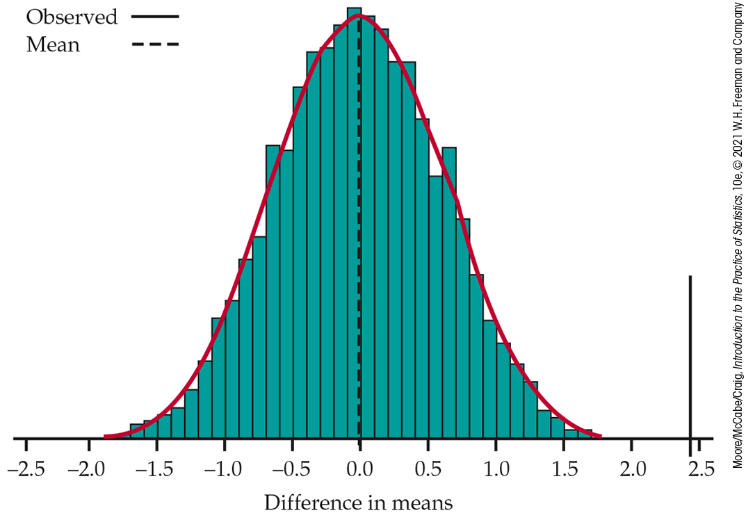
Figure 16.28 The permutation distribution for the mean difference (moon days minus other days) from 10,000 paired resamples from the data in Table 16.2, Example 16.18.
The permutation distribution in Figure 16.28 is close to Normal, as a Normal quantile plot confirms. The matched pairs t test is therefore reliable and agrees with the permutation test that the P-value is very small.
Permutation test for the significance of a relationship.
Permutation testing can be used to test the significance of a relationship between two variables. For example, in Example 16.13, we looked at the relationship between price and rating of laundry detergents.
The null hypothesis is that there is no relationship. In that case, prices are assigned to detergents for reasons that have nothing to do with rating. We can resample in a way consistent with the null hypothesis by permuting the observed ratings among the detergents at random.
Take the correlation as the test statistic. For every resample, calculate the correlation between the prices (in their original order) and ratings (in the reshuffled order). The P-value is the proportion of the resamples with correlation larger than the original correlation.
When can we use permutation tests?
We can use a permutation test only when we can see how to resample in a way that is consistent with the study design and with the null hypothesis. We now know how to do this for the following types of problems:
- Two-sample problems when the null hypothesis says that the two populations are identical. We may wish to compare population means, proportions, standard deviations, or other statistics. You may recall from Section 7.3 that traditional tests for comparing population standard deviations work very poorly. Permutation tests are a much better choice.
- Matched pairs designs when the null hypothesis says that there are only random differences within pairs. A variety of comparisons is again possible.
- Relationships between two quantitative variables when the null hypothesis says that the variables are not related. The correlation is the most common measure of association, but it is not the only one.
These settings share the characteristic that the null hypothesis
specifies a simple situation such as two identical populations or
two unrelated variables. We can see how to resample in a way that
matches these situations.
![]() Permutation tests can’t be used for testing hypotheses about a
single population, comparing populations that differ even under
the null hypothesis, or testing general relationships.
In these settings, we don’t know how to resample in a way that
matches the null hypothesis. Researchers are developing resampling
methods for these and other settings, so stay tuned.
Permutation tests can’t be used for testing hypotheses about a
single population, comparing populations that differ even under
the null hypothesis, or testing general relationships.
In these settings, we don’t know how to resample in a way that
matches the null hypothesis. Researchers are developing resampling
methods for these and other settings, so stay tuned.
When we can’t do a permutation test, we can often calculate a
bootstrap confidence interval instead. If the confidence interval
fails to include the null hypothesis value, then we reject
Section 16.5 SUMMARY
- Permutation tests are significance tests based on permutation resamples drawn at random from the original data. Permutation resamples are drawn without replacement, in contrast to bootstrap samples, which are drawn with replacement.
- Permutation resamples must be drawn in a way that is consistent with the null hypothesis and with the study design. In a two-sample design, the null hypothesis says that the two populations are identical. Resampling randomly reassigns observations to the two groups. In a matched pairs design, randomly permute the two observations within each pair separately. To test the hypothesis of no relationship between two variables, randomly reassign values of one of the two variables.
- The permutation distribution of a suitable statistic is formed by the values of the statistic in a large number of resamples. Find the P-value of the test by locating the original value of the statistic on the permutation distribution.
- When they can be used, permutation tests have great advantages. They do not require specific population shapes such as Normality. They apply to a variety of statistics, not just to statistics that have a simple distribution under the null hypothesis. They can give very accurate P-values, regardless of the shape and size of the population (if enough permutations are used).
- It is often useful to give a confidence interval along with a test. To create a confidence interval, we no longer assume that the null hypothesis is true, so we use bootstrap resampling rather than permutation resampling.
Section 16.5 EXERCISES
-
16.53 Marketing smartphones. You received two prototypes of a new smartphone and designed an experiment to help decide which one to market. Forty students were each randomly assigned to use one of the two phones for two weeks. Their overall satisfaction with the phone was recorded on a subjective scale with a range of 1 to 100. Outline the steps needed to compare the means for the two smartphones using a permutation test.
-
16.54 Marketing smartphones (continued). Refer to the previous exercise. Suppose that you had each of the 40 students use both smartphones. Each is used for one week, and the order is randomly determined. Outline the steps needed to compare the means for the two smartphones using a permutation test.
-
16.55 Features of smartphones. Refer to Exercise 16.53. Before asking the students to provide an overall satisfaction rating, you asked them to provide ratings, using the same scale of 1 to 100, for several features of the smartphone. Two of these were satisfaction with the touchscreen and satisfaction with the Internet connectivity. Are these two features correlated? Outline the steps needed to evaluate the relationship between these two variables for each of the smartphones using a permutation test.
-
16.56 Compare the correlations. Refer to the previous exercise. Suppose that you calculate the correlation between the satisfaction of these two features for each phone. Outline the steps needed to compare these two correlations using a permutation test.
-
16.57 A small-sample permutation test. For this exercise, perform a permutation test by hand for a small random subset of the DRP data (Example 16.15, page 16-39). Here are the data:

Treatment group 57 67 Control group 53 42 42 37 -
Calculate the difference in means
-
Resample: Start with the six scores and choose an SRS of two scores to form the treatment group for the first resample. You can do this by labeling the scores from 1 to 6 and using consecutive random digits from Table B or by rolling a die. Using either method, be sure to skip repeated digits. A resample is an ordinary SRS, without replacement. The remaining four scores are the control group. What is the difference in group means for this resample?
-
Repeat part (b) 20 times to get 20 resamples and 20 values of the statistic. Make a histogram of the distribution of these 20 values. This is the permutation distribution for your resamples.
-
What proportion of the 20 statistic values were equal to or greater than the original value in part (a)? You have just estimated the one-sided P-value for the original 6 observations.
-
For this small data set, there are only 15 possible permutations of the data. As a result, we can calculate the exact P-value by counting the number of permutations with a statistic value greater than or equal to the original value and then dividing by 15. What is the exact P-value here? How close was your estimate?
-
-
16.58 Product labels with animals? Participants in a study were asked to indicate their attitude toward a product on a seven-point scale (from

Group Brand attitude Primed 2 2 3 3 3 4 4 4 4 4 4 4 4 4 4 5 5 5 5 5 5 5 Nonprimed 1 1 2 2 3 3 3 3 3 3 3 3 3 3 3 3 4 4 4 5 -
Examine the scores of each group graphically. Is it appropriate to use the two-sample t procedures? Explain your answer.
-
Perform the two-sample t test to compare the group means. Use a two-sided alternative hypothesis and a significance level of 5%.
-
Perform a permutation test to compare the group means. Summarize your results and conclusions.
-
Write a short summary comparing your results in parts (b) and (c). Which method do you recommend for these data? Give reasons for your answer.
-
-
16.59 Low-calorie sweeteners. Examples 7.18 and 7.19 (page 407) examine data on an experiment to compare weight change in subjects who were asked to consume a sweetened beverage in addition to their normal diet. The sweetened beverage was sweetened with either saccharin or sucralose. In Example 7.19, the following data were analyzed:

Group Weight change (kg) Saccharin 0.5 3.0 4.2 2.3 3.3 Sucralose 0.1 1.2 -
State appropriate null and alternative hypotheses for these data.
-
Report the result of the pooled two-sample t test.
-
Perform a permutation test to compare the two means and report the results. Compare the P-value for this test with the P-value for the t test in part (b).
-
Find a BCa confidence interval for the difference in means. How is this interval related to your results in part (c)?
-
-
16.60 Standard deviation of the estimated P-value. The estimated P-value for the DRP study (Example 16.16, page 16-40) based on 1000 resamples is
-
 16.61 When is a permutation test valid?
You want to test the equality of the means of two populations.
Sketch density curves for two populations for which
16.61 When is a permutation test valid?
You want to test the equality of the means of two populations.
Sketch density curves for two populations for which
-
a permutation test is valid but a t test is not.
-
both permutation and t tests are valid.
-
a t test is valid but a permutation test is not.
-
-
16.62 Testing the correlation between BMI and physical activity. In Exercise 16.47 (page 16-37), we assessed the significance of the correlation between BMI and physical activity by creating bootstrap confidence intervals. If a 95% confidence interval does not cover 0, the observed correlation is significantly different from 0 at the

-
16.63 Assessing a summer language institute. Exercise 7.105 (page 447) gives data on a study of the effect of a summer language institute on the ability of high school language teachers to understand spoken French. This is a matched pairs study, with scores for 20 teachers at the beginning (pretest) and end (posttest) of the institute. We conjecture that the posttest scores are higher on the average.

-
Carry out the matched pairs t test. That is, state hypotheses, calculate the test statistic, and give the P-value of the test statistic.
-
Make a Normal quantile plot of the gains:
-
Carry out the permutation test for the difference in means in a matched pairs setting, using 9999 resamples. The Normal quantile plot shows that the permutation distribution is reasonably Normal. What is the P-value for the permutation test? Do your tests in parts (a) and (c) lead to the same practical conclusion?
-
-
16.64 Compare the medians. Refer to the previous exercise. Use a permutation test to compare the medians. Write a short summary of your results and conclusions. Include a comparison of what you found here with what you found in the previous exercise.
-
16.65 Testing the correlation between price and rating. Example 16.14 (page 16-34) uses the bootstrap to find a confidence interval for the correlation between price and rating for 24 laundry detergents. Let’s use a permutation test to examine this correlation.

State the null and alternative hypotheses.
-
Perform a permutation test based on the sample correlation. Report the P-value and draw a conclusion.
-
16.66 Comparing mpg calculations. Exercise 7.25 (page 408) gives data on a comparison of driver and computer mpg calculations. This is a matched pairs study, with mpg values for 20 fill-ups.

-
Carry out the matched pairs t test. That is, state hypotheses, calculate the test statistic, and give its P-value.
-
A permutation test can help check the t test result. Carry out the permutation test for the difference in means in a matched pairs setting, using 10,000 resamples. Does this test and the test in part (a) lead to the same practical conclusion?
-
-
16.67 Comparing standard deviations.
In
Example 12.17
(page 620),
the modified Levene’s test was used to compare standard
deviations. Let’s now consider performing a permutation test
using the F statistic (the ratio of the largest and
smallest sample variances) as your statistic. What do you
conclude? Are the two tests comparable?

-
16.68 Comparing serum retinol levels. The formal medical term for vitamin A in the blood is serum retinol. Serum retinol has various beneficial effects, such as protecting against fractures. Medical researchers working with children in Papua New Guinea asked whether recent infections reduce the level of serum retinol. They classified children as recently infected or not on the basis of other blood tests and then measured serum retinol. Of the 90 children in the sample, 55 had been recently infected. Table 16.3 gives the serum retinol levels for both groups, in micromoles per liter.11

-
The researchers are interested in the proportional reduction in serum retinol. Verify that the mean for infected children is 0.620 and that the mean for uninfected children is 0.778.
-
There is no standard test for the null hypothesis that the ratio of the population means is 1. We can do a permutation test on the ratio of sample means. Carry out a one-sided test and report the P-value. Briefly describe the center and shape of the permutation distribution. Why do you expect the center to be close to 1?
Table 16.3 Serum retinol levels
Not infected Infected 0.59 1.08 0.88 0.62 0.46 0.39 0.68 0.56 1.19 0.41 0.84 0.37 1.44 1.04 0.67 0.86 0.90 0.70 0.38 0.34 0.97 1.20 0.35 0.87 0.35 0.99 1.22 1.15 1.13 0.67 0.30 1.15 0.38 0.34 0.33 0.26 0.99 0.35 0.94 1.00 1.02 1.11 0.82 0.81 0.56 1.13 1.90 0.42 0.83 0.35 0.67 0.31 0.58 1.36 0.78 0.68 0.69 1.09 1.06 1.23 1.17 0.35 0.23 0.34 0.49 0.69 0.57 0.82 0.59 0.24 0.41 0.36 0.36 0.39 0.97 0.40 0.40 0.24 0.67 0.40 0.55 0.67 0.52 0.23 0.33 0.38 0.33 0.31 0.35 0.82 -
-
16.69 Methods of resampling. In Exercise 16.68, we did a permutation test for the hypothesis “no difference between infected and uninfected children,” using the ratio of mean serum retinol levels to measure “difference.” We might also want a bootstrap confidence interval for the ratio of population means for infected and uninfected children. Describe carefully how the resampling differs for the permutation test and for the bootstrap.
-
16.70 Listening to podcasts. A 2015 Edison Research study asked U.S. individuals age 12 and older whether or not they had ever listened to a podcast. The survey was repeated with different users in 2020.12 For the 2015 survey, 660 of the 2002 people surveyed reported that they had listened to at least one audio podcast. In the 2020 survey, the results were 827 of the 1502 survey participants. We want to use these sample data to test equality of the population proportions of successes. Carry out a permutation test. Describe the permutation distribution. Give the P-value and report your conclusion.
-
16.71 Sex and GPA.
In
Exercise 16.45
(page 16-37), we used the bootstrap to compare the mean GPA scores for men
and women.

-
Use permutation methods to compare the means for men and women.
-
Use permutation methods to compare the standard deviations for men and women.
-
Write a short paragraph summarizing your results and conclusions.
-
-
16.72 The effect of outliers (continued). In Exercise 16.52 (page 16-38), we studied the effect of outliers on the bootstrap distribution and confidence intervals. For this exercise, perform the permutation test without the three patients with very small differences and compare the results with those in Example 16.18. Discuss any differences you find and how you would report the results to the nursing home staff.