7.3 Sample Size Calculations
In this section, we focus on a very important issue when planning a
study: choosing the sample size.
![]() A wise user of statistics does not plan for inference without at the
same time planning data collection.
We describe sample size procedures for both confidence intervals and
significance tests. While the actual formulas are a bit technical, only
a general understanding of the process is necessary. We can rely on
software to do the heavy lifting.
A wise user of statistics does not plan for inference without at the
same time planning data collection.
We describe sample size procedures for both confidence intervals and
significance tests. While the actual formulas are a bit technical, only
a general understanding of the process is necessary. We can rely on
software to do the heavy lifting.
Sample size for confidence intervals
We can arrange to have both high confidence and a small margin of error by choosing an appropriate sample size. Let’s first focus on the one-sample t confidence interval. Its margin of error is
In addition to the confidence level C, which determines
We’ll call this guessed value
following the 68–95–99.7 rule. It is always better to use a value of the standard deviation that is a little larger than what is expected. This may result in a sample size that is a little larger than needed, but it helps avoid the situation where the resulting margin of error is larger than desired.
Given the desired margin of error m and a guess for s,
we can find the sample size by plugging these values into the margin
of error formula and solving for n. In fact, we did this in
Chapter 6 (page 340). The one complication here is that
Finding the smallest sample size n that satisfies this requirement can be done using the following iterative search:
-
Get an initial sample size by replacing
-
Use this sample size to obtain
- If the requirement is satisfied, then this n is the needed sample size. If the requirement is not satisfied, increase n by 1 and return to Step 2.
Notice that this method makes no reference to the size of the population. It is the size of the sample that determines the margin of error. The size of the population does not influence the sample size we need as long as the population is much larger than the sample.
Example 7.23 Planning a study of a robot delivery service.
In
Example 7.1
(page 387), we
calculated a 95% confidence interval for the average delivery time,
in minutes, for a delivery robot service to bring you lunch ordered
from Cosi. The margin of error based on an SRS of
The sample standard deviation in
Example 7.1
is
-
For an initial n, we replace
Round up to get
-
We now check to see if this sample size satisfies the requirement when we switch back to
This is larger than
-
The following table summarizes these calculations for some larger values of n.
n 36 5.075 37 5.001 38 4.930
The requirement is first satisfied when
Figure 7.20 shows the Minitab input window used to do these calculations. Because the default confidence level is 95%, only the desired margin of error m and the estimate for s need to be entered. The software does the rest once you click OK.
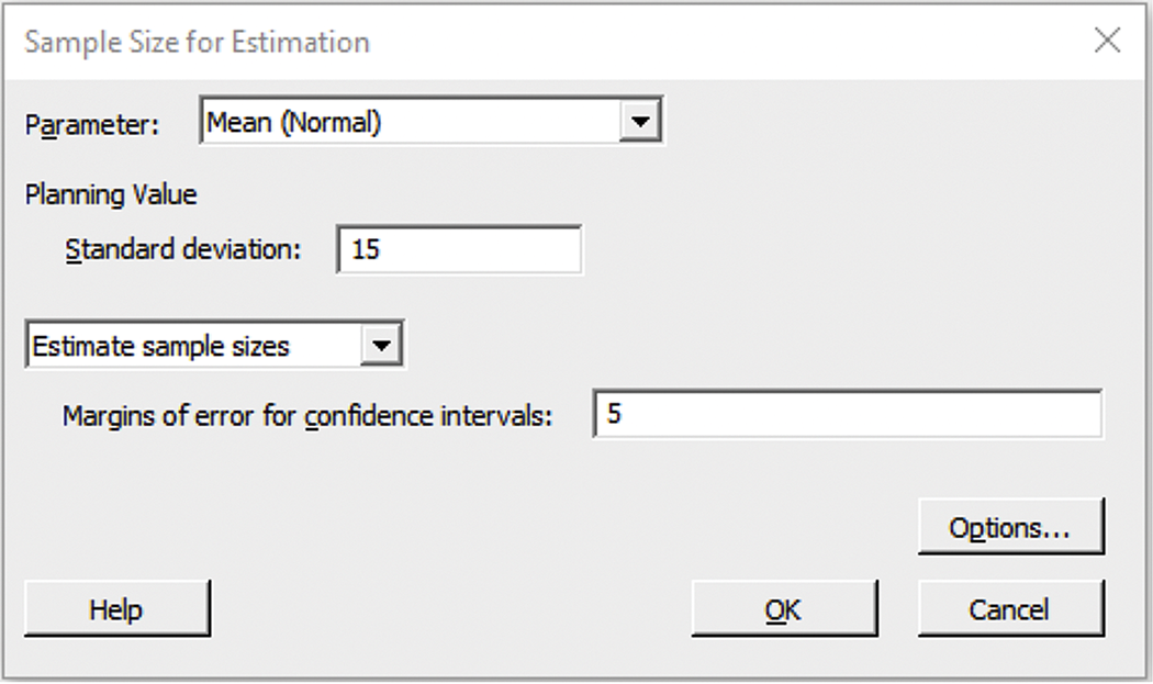
Figure 7.20 Minitab input window used to compute the sample size for a desired margin of error, Example 7.23.
Note that the
![]() This does not guarantee that the margin of error for the collected
sample will be less than 5 minutes.
That is because the sample standard deviation s varies from
sample to sample, and these calculations are treating it as a fixed
quantity. If you want stronger control of the margin of error, more
advanced sample size procedures ask you to also specify the
probability of obtaining a
margin of error less than the desired value. For the current approach,
this probability is roughly 50%. For a probability closer to 100%, the
sample size will need to be larger. For example, if we wanted this
probability to be roughly 80%, we’d perform these calculations in SAS
using the commands
This does not guarantee that the margin of error for the collected
sample will be less than 5 minutes.
That is because the sample standard deviation s varies from
sample to sample, and these calculations are treating it as a fixed
quantity. If you want stronger control of the margin of error, more
advanced sample size procedures ask you to also specify the
probability of obtaining a
margin of error less than the desired value. For the current approach,
this probability is roughly 50%. For a probability closer to 100%, the
sample size will need to be larger. For example, if we wanted this
probability to be roughly 80%, we’d perform these calculations in SAS
using the commands
proc power;
  onesamplemeans CI=t stddev=15.0 halfwidth=5
            probwidth=0.80 ntotal=.;
run;
The needed sample size increases from
![]() Unfortunately, the actual number of usable observations is often
less than that planned at the beginning of a study.
This is particularly true of data collected in surveys or studies that
involve a time commitment from the participants. Careful study
designers often assume a nonresponse rate or dropout rate that
specifies what proportion of the originally planned sample will fail
to provide data. We use this information to calculate the sample size
to be used at the start of the study. For example, if a survey were
planned needing
Unfortunately, the actual number of usable observations is often
less than that planned at the beginning of a study.
This is particularly true of data collected in surveys or studies that
involve a time commitment from the participants. Careful study
designers often assume a nonresponse rate or dropout rate that
specifies what proportion of the originally planned sample will fail
to provide data. We use this information to calculate the sample size
to be used at the start of the study. For example, if a survey were
planned needing
These sample size calculations also do not account for collection costs. In practice, taking observations costs time and money. There are times when the required sample size may be impossibly expensive. In those situations, one might consider a larger margin of error and/or a lower confidence level to be acceptable.
Check-in
-
7.21 How do design choices change the sample size? Refer to Example 7.23. For each of the following changes, state whether the needed sample size will increase or decrease and explain your reasoning.
-
The desired margin of error is 7.5 minutes rather than 5 minutes.
A 90% rather than 95% confidence level is used.
-
We use
-
-
7.22 How many postings to sample? For Check-in question 7.1 (page 386), a random sample of
For the two-sample t confidence interval, the margin of error is
A similar type of iterative search can be used to determine the sample
sizes
An alternative approach is to consider that the standard deviations and sample sizes are the same, so the margin of error is
and the degrees of freedom are
Example 7.24 Planning a new blood pressure study.
In Example 7.22 (page 426), we calculated a 90% confidence interval for the mean difference in blood pressure. The 90% margin of error was roughly 5.6 mm Hg, which was relatively large. Suppose that a new study is being planned and the desired margin of error at 90% confidence is 2.8 mm Hg. How many subjects per group do we need?
The pooled sample standard deviation in Example 7.22 is 7.385. To be a bit conservative, we’ll guess that the two population standard deviations are both 8.0. We now implement the same iterative search method using the two-sample margin of error formula.
-
For an initial n, we replace
We round up to get
-
The following table summarizes the margin of error for this and some larger values of n:
| n |
|
|---|---|
| 45 | 2.834 |
| 46 | 2.801 |
| 47 | 2.770 |
The margin of error is smaller than 2.8 mm Hg when
proc power;
twosamplemeans CI=diff alpha=0.1 stddev=8
              halfwidth=2.8
               probwidth=0.50 npergroup=.;
run;
This sample size is roughly 4.5 times the sample size used in Example 7.22. This researcher may not be able to recruit a sample this large. We should therefore consider alternatives such as a larger desired margin of error.
Check-in
-
7.23 Would we need a larger sample size? Refer to Example 7.24. For each of the following changes, state whether the needed sample size will increase or decrease and explain your reasoning.
-
The desired margin of error is 3 mm Hg instead of 2.8 mm Hg.
A 95% rather than 90% confidence level is used.
-
We use
-
-
7.24 Planning a new calcium study. Refer to Example 7.24. What is the required sample size if the goal is have the 95% margin of error no more than 5 mm Hg? Use
Power of a significance test
The power of a statistical test measures its ability to detect deviations from the null hypothesis. In practice, we carry out a significance test in the hope of showing that the null hypothesis is false. The higher the power, the more likely this will occur. Unfortunately, because of inadequate planning, researchers frequently fail to find evidence for the effects that they believe to be present. This is often the result of an inadequate sample size. Power calculations performed prior to running the experiment help avoid this occurrence and ensure that the sample size is sufficiently large to answer the research question.
Just like the margin of error, the power of a significance test depends on various study-specific factors. The factors and how they impact power are as follows:
-
Significance level
-
Population standard deviation(s). More variation
means more uncertainty (less precision) about the mean(s). With more
uncertainty, we are less likely to reject
- Sample size(s). More data will provide more information about the mean(s) (smaller standard error) and thus a greater chance of distinguishing the alternative.
-
The alternative. The further the alternative is
from the null hypothesis, the easier it is to distinguish it from
The margin of error depends on the first three factors. Any change in these factors that increases the power of a significance test also results in a smaller margin of error. This is due to the close relationship between significance tests and confidence intervals.
As for the fourth factor, we usually rely on subject-specific
knowledge to choose this value. It is typically the smallest departure
from
There are times, however, when the choice of the alternative is not
clear-cut. In these situations, we commonly consider the
effect
size, which is the departure from
Figure 7.21
visually displays these two steps for a one- or two-sample
t test under the greater-than alternative. The distribution of
the test statistic under
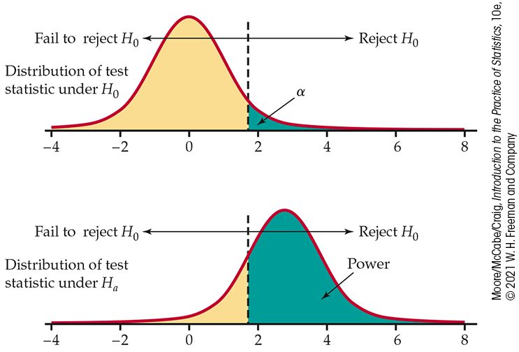
Figure 7.21 Visual for
computing power under the greater-than alternative. The sampling
distributions of the test statistic under both
We just need to provide the four study-specific factors and let the software do the technical calculations. When considering the effect size but working with software that does not include effect size, set the alternative equal to the effect size and set the population standard deviation equal to 1.
We’ll now run through both one- and two-sample examples.
Example 7.25 Is the sample size large enough?
Recall
Example 7.2
(page 389) on
the average delivery time from Cosi to your dormitory by a robot
delivery service. Your roommate eats lunch at a different time and
wants to perform a similar study. She also wants to test if the
average delivery time is larger than 15 minutes but additionally
wants to be very certain her study will reject
To answer this, we compute the power of the one-sample t test at the 5% significance level for
against the alternative that
Figure 7.22
shows Minitab output for this power calculation. The power when
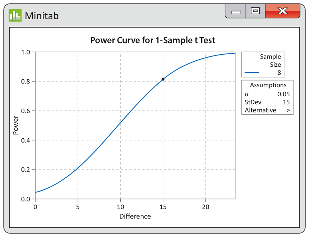
Figure 7.22 Minitab output (a power curve) for the one-sample calculation, Example 7.25.
Check-in
-
7.25 Power for other values of
-
-
7.26 How is power affected? Refer to Example 7.25.
-
If your roommate used
-
If your roommate used
-
For the two-sample power calculation, we consider only the common case
where the null hypothesis is “no difference,”
Example 7.26 Planning a new study of calcium versus placebo groups.
In
Example 7.19
(page 421), we
examined the effect of calcium on blood pressure by comparing the
means of a treatment group and a placebo group using a pooled
two-sample t test. The P-value was 0.059, failing to
achieve the usual standard of 0.05 for statistical significance.
Suppose that we wanted to plan a new study that would provide
convincing evidence—say, at the 0.01 level—with high probability.
Let’s examine a study design with 45 subjects in each group
Figure 7.23
shows the JMP power calculator for the two-sample t test. You
input values for
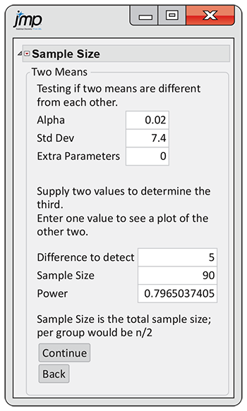
Figure 7.23 JMP input/output window for the two-sample power calculation, Example 7.26.
![]()
The power window in
Figure 7.23
shows that the power under these settings in 79.7%. If we judge this
probability to be high enough, we can proceed with recruitment.
However, given that there is a chance some subjects will dropout or
not follow the protocol, we may want to recruit a larger sample,
such as
These two examples focused on determining the power for a given sample size. Calculators such as the one in Figure 7.21 can also be used to determine a sample size for a selected level of power and alternative or the alternative it can detect at a given level of power for a given sample size. This makes these calculators very flexible and informative.
Check-in
-
7.27 Power and the choice of alternative. If you were to repeat the calculation in Example 7.26 for the two-sided alternative, would the power increase or decrease? Explain your answer.
-
7.28 Power and the standard deviation. If the true population standard deviation were 8 instead of the 7.4 hypothesized in Example 7.26, would the power increase or decrease? Explain.
Section 7.3 SUMMARY
-
The sample size required to obtain a confidence interval of a population mean
-
where
-
For a two-sample confidence interval of the difference in means, the necessary sample sizes can be obtained using a similar constraint. Most often it is assumed that the standard deviations and sample sizes are the same.
-
The power of the one- and two-sample t tests involves the noncentral t distributions. Calculations involving these distributions are not practical by hand but are easy with software.
-
To compute the power, the researcher must provide the significance level
Section 7.3 EXERCISES
-
7.66 What’s wrong? For each of the following statements, explain what is wrong and why.
-
Doubling the sample size means the margin of error for a population mean
-
When testing
-
Increasing sample size increases the power and decreases the probability of a Type I error.
-
When testing
-
-
7.67 Starting salaries. In a recent survey by the National Association of Colleges and Employers, the average starting salary for college graduates with a computer and information sciences degree was reported to be $81,292.43 You are planning to do a survey of starting salaries for recent computer science majors from your university.
-
Using an estimated standard deviation of $12,100, what sample size do you need to have a margin of error equal to $5000 with 95% confidence?
-
Suppose that, in the setting of part (a), you have the resources to contact 30 recent graduates. If all respond, will your margin of error be larger or smaller than $5000? What if only 80% respond? Verify your answers by performing the calculations.
-
-
7.68 Apartment rental rates. You hope to rent an unfurnished one-bedroom apartment in Washington, DC, next year. You call a friend who lives there and ask him to give you an estimate of the mean monthly rate. Having taken a statistics course recently, the friend asks about your desired margin of error and confidence level for this estimate. He also tells you that the standard deviation of monthly rents for one-bedroom apartments is about $640.
-
For 95% confidence and a margin of error of $200, how many apartments should your friend randomly sample from Realtor.com?
-
Suppose that you want the margin of error to be no more than $100. How many apartments should your friend sample?
-
Why is the sample size in part (b) not just four times larger than the sample size in part (a)?
-
-
7.69 More on apartment rental rates. Refer to the previous exercise. Will the 95% confidence interval include approximately 95% of the rents of all unfurnished one-bedroom apartments in this area? Explain why or why not.
-
7.70 Accuracy of a laboratory scale. To assess the accuracy of a laboratory scale, a standard weight known to weigh 10 grams is weighed repeatedly. The scale readings are Normally distributed, with unknown mean. (The mean is 10 grams if the scale has no bias.) The standard deviation of the scale readings in the past has been 0.0013 gram.
-
The weight is measured five times. The mean result is 10.0009 grams. Give a 98% confidence interval for the mean of repeated measurements of the weight.
-
How many measurements must be averaged to get an expected margin of error no more than 0.001 with 98% confidence?
-
-
7.71 Accuracy of a laboratory scale, continued. Refer to the previous exercise. Suppose that instead of a confidence interval, the researchers want to perform a test (with
-
What sample size n is necessary to have at least 90% power when the alternative mean is
-
Suppose the researchers can only perform a maximum of
-
Verify your answer in part (b) by computing the power when
-
-
7.72 Sample size calculations. You are designing a study to test the null hypothesis that
-
7.73 Power of the comparison of DXA machine operators. Suppose that the bone researchers in Exercise 7.29 (page 409) want to be able to detect an alternative mean difference of 0.002. Find the power for this alternative for a sample size of 20 patients. Make sure to explain the reasoning for your choice of standard deviation in these calculations.
-
7.74 Determining the sample size. In Example 7.25 (page 439), we determined the power of detecting
-
7.75 Changing the significance level. In Example 7.26 (page 440), we assessed the power of a new study of calcium on blood pressure, assuming
-
Would the power increase or decrease? Explain your answer in terms someone unfamiliar with power calculations can understand.
Verify your answer by computing the power.
-
-
7.76 Planning a study to compare tree size. In Exercise 7.57 (page 432), DBH data for longleaf pine trees in two parts of the Wade Tract are compared. Suppose that you are planning a similar study in which you will measure the diameters of longleaf pine trees. Based on Exercise 7.57, you are willing to assume that the standard deviation for both halves is 20 cm. Suppose that a difference in mean DBH of 10 cm or more would be important to detect. You will use a t statistic and a two-sided alternative for the comparison.
-
Find the power if you randomly sample 20 trees from each area to be compared.
-
Repeat the calculations for 60 trees in each sample.
-
If you had to choose between the 20 and 60 trees per sample, which would you choose? Give reasons for your answer.
-
-
 7.77 More on planning a study to compare tree size.
Refer to the previous exercise. Find the two standard deviations
from
Exercise 7.57. Do the same for the data in
Exercise 7.58, which is a similar setting. These are somewhat smaller than
the assumed value that you used in the previous exercise.
Explain why it is generally a better idea to assume a standard
deviation that is larger than you expect than one that is
smaller. Repeat the power calculations for some other reasonable
values of
7.77 More on planning a study to compare tree size.
Refer to the previous exercise. Find the two standard deviations
from
Exercise 7.57. Do the same for the data in
Exercise 7.58, which is a similar setting. These are somewhat smaller than
the assumed value that you used in the previous exercise.
Explain why it is generally a better idea to assume a standard
deviation that is larger than you expect than one that is
smaller. Repeat the power calculations for some other reasonable
values of
-
7.78 Planning a study to compare ad placement. Refer to Exercise 7.56 (page 431), where we compared trustworthiness ratings for ads from two different publications. Suppose that you are planning a similar study using two different publications that are not expected to show the differences seen when comparing the Wall Street Journal with the National Enquirer. You would like to detect a difference of 1.5 points using a two-sided significance test with a 5% level of significance. Based on Exercise 7.56, it is reasonable to use 1.6 as the value of the common standard deviation for planning purposes.
-
What is the power if you use sample sizes similar to those used in the previous study—for example, 65 for each publication?
Repeat the calculations for 100 in each group.
-
What sample size would you recommend for the new study?
-