11.2 A Case Study
In this section, we illustrate multiple regression by analyzing the data
from the study described in
Example 11.1.
There are data for
Before starting the analysis, we must first consider the extent to which our results can be generalized. For this study, all the available data are being analyzed. There is no random sampling from the population of science majors. In this type of setting, we often justify the use of inference by viewing the data as coming from some sort of process. Here, we consider this collection of students as a sample of all the science majors who will attend this university. Still, opinions may vary as to the extent to which these data can be considered an SRS sample of future students. For example, schools seem to consistently brag that their new batch of first-year students is the smartest and most accomplished group they’ve ever had.
Preliminary analysis
As with any other statistical analysis, we begin our multiple regression with a careful examination of the data. We first look at each variable separately, and then we look at relationships among the variables. In both cases, we continue our practice of combining plots and numerical descriptions. We use a mix of JMP, Excel, and Minitab to illustrate the outputs that are given by most software.
Example 11.3 Numerical summaries of each variable.
![]()

Means, standard deviations, and minimum and maximum values appear in
Figure 11.2. The minimum value for high school mathematics (HSM) appears to be
rather extreme; it is 4.51 standard deviations below the mean
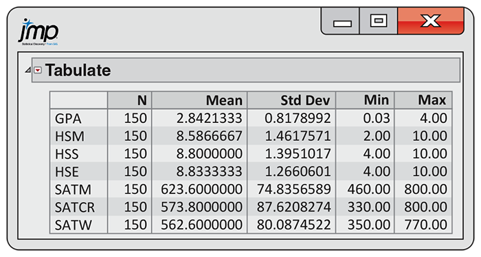
Figure 11.2 Descriptive statistics for the academic success case study, Example 11.3.
![]()
The mean for the SATM score is higher than the means for the Critical Reading (SATCR) and Writing (SATW) scores, as we might expect for a group of science majors. The three SAT standard deviations are all about the same.
Although mathematics scores were higher on the SAT, the means and standard deviations of the three high school grade variables are very similar. Because the level and difficulty of high school courses vary within and across schools, this may not be that surprising. The mean GPA is 2.842 on a four-point scale, with standard deviation 0.818.
It is often easier to study a variable visually than to look at a set of numerical summaries. For quantitative variables, we can use boxplots and histograms to examine the shapes of their distributions and identify extreme values. For categorical variables, we can use bar plots or pie charts.
Example 11.4 Graphical summary of each variable.
![]()
Because the variables GPA, SATM, SATCR, and SATW have many possible values, we could use boxplots or histograms to examine their shapes. For GPA (not shown), the distribution is strongly skewed to the left so that its minimum value does not look as extreme anymore.
The high school grade variables HSM, HSS, and HSE take only integer
values. The bar plots using relative frequencies are shown in
Figure 11.3. The distributions are all skewed, with a large proportion of high
grades
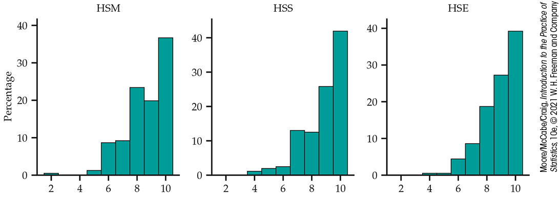
Figure 11.3 Bar plots using relative frequencies, Example 11.4.
The purpose of examining these numerical and visual summaries is to
understand the features of each variable before attempting to use it
in a complicated model.
![]() Extreme values of any variable should be noted and checked for
accuracy. If they are found to be correct, the cases with these values should
be carefully examined to see if they are truly exceptional and perhaps
do not belong in the same analysis with the other cases. We will see
that when our data are examined in this way, no obvious problems are
evident.
Extreme values of any variable should be noted and checked for
accuracy. If they are found to be correct, the cases with these values should
be carefully examined to see if they are truly exceptional and perhaps
do not belong in the same analysis with the other cases. We will see
that when our data are examined in this way, no obvious problems are
evident.
It should also be noted that this preliminary analysis did not involve
checks of Normality using Normal quantile plots. Just as with simple
linear regression,
![]() the multiple regression model does not require any of these
observed distributions to be Normal. Only the deviations of the responses y from their means are
assumed to be Normal. This condition can be assessed only after we’ve
fit the model.
the multiple regression model does not require any of these
observed distributions to be Normal. Only the deviations of the responses y from their means are
assumed to be Normal. This condition can be assessed only after we’ve
fit the model.
Check-in
-
11.3 Examining the distributions of the other variables. Use boxplots or histograms to examine the distributions of GPA, SATM, SATCR, and SATW. Describe the shapes and comment on any extreme values.

Relationships between pairs of variables
The second step in our analysis is to examine the relationships between all pairs of variables. Scatterplots and correlations are our tools for studying two-variable relationships.
Example 11.5 Examining the correlations between pairs of variables.
![]()
The correlations appear in
Figure 11.4. As we might expect, high school math and science grades have the
highest correlation with GPA
Some software output includes the P-value for the test of
the null hypothesis that the population correlation is 0 versus the
two-sided alternative for each pair. When you have a large sample
size, this information is not that helpful as even somewhat weak
associations are found to be statistically significant. For example,
with
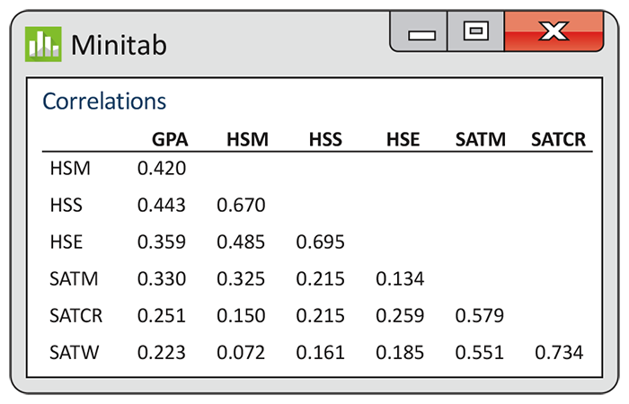
Figure 11.4 Correlations among case study variables, Example 11.5.
It is important to keep in mind that, by examining pairs of variables,
we are seeking a better understanding of the data.
![]() The fact that the correlation of a particular explanatory variable
with the response variable does not achieve statistical significance
does not necessarily imply that it will not be a useful (and
statistically significant) predictor in a multiple regression
model.
The fact that the correlation of a particular explanatory variable
with the response variable does not achieve statistical significance
does not necessarily imply that it will not be a useful (and
statistically significant) predictor in a multiple regression
model.
Numerical summaries such as correlations are useful, but plots are
generally more informative when seeking to understand data. Plots tell
us whether the numerical summary gives a fair representation of the
data. For a multiple regression, each pair of variables should be
plotted. For the seven variables in our case study, this means that we
should examine 21 plots. In general, there are
![]() Multiple regression is a complicated procedure. If we do not do the
necessary preliminary work, we are in serious danger of producing
useless or misleading results.
Multiple regression is a complicated procedure. If we do not do the
necessary preliminary work, we are in serious danger of producing
useless or misleading results.
Check-in
-
11.4 Pairwise relationships among variables in the GPA data set. Most statistical software packages have the option to create a “scatterplot matrix” of all
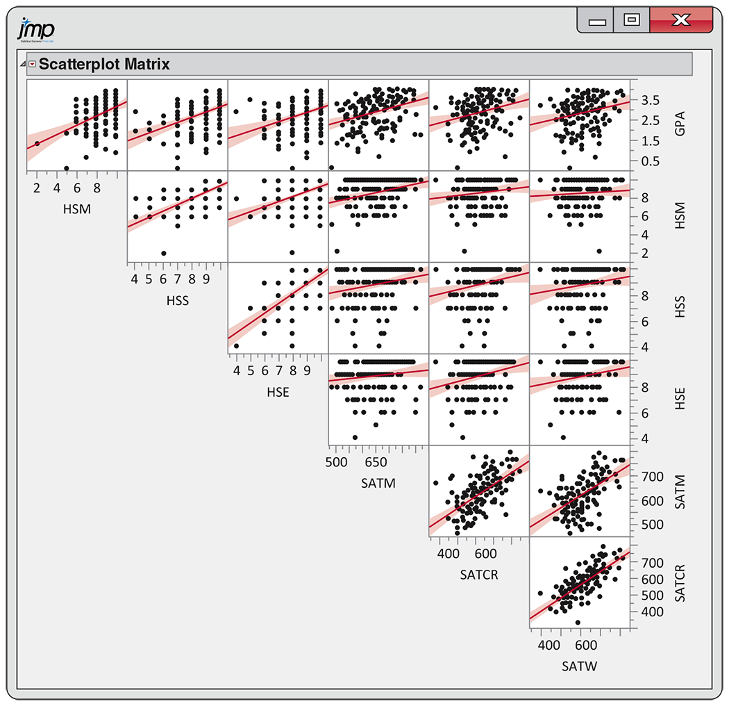
Figure 11.5 Scatterplot matrix for the academic success case study, including the least-squares lines, Check-in question 11.4.
Fitting a multiple regression model
![]()
To explore the relationship between the explanatory variables and our response variable GPA, we run several multiple regressions. The explanatory variables fall into three classes. High school grades are represented by HSM, HSS, and HSE; standardized tests are represented by the three SAT scores; and sex of the student is represented by Sex. We begin our analysis by using the high school grades to predict GPA.
Example 11.6 Regression on high school grades.
![]()
Figure 11.6
gives the multiple regression output when using the three high
school grades as explanatory variables. The output contains an ANOVA
table, some additional fit statistics, and information about the
parameter estimates. Because there are
The ANOVA F statistic is 14.35, with a P-value of
the F statistic has an F(3, 146) distribution. According to this distribution, the chance of obtaining an F statistic of 14.35 or larger is less than 0.0001. Therefore, we conclude that at least one of the three regression coefficients for the high school grades is different from 0 in this population regression equation.
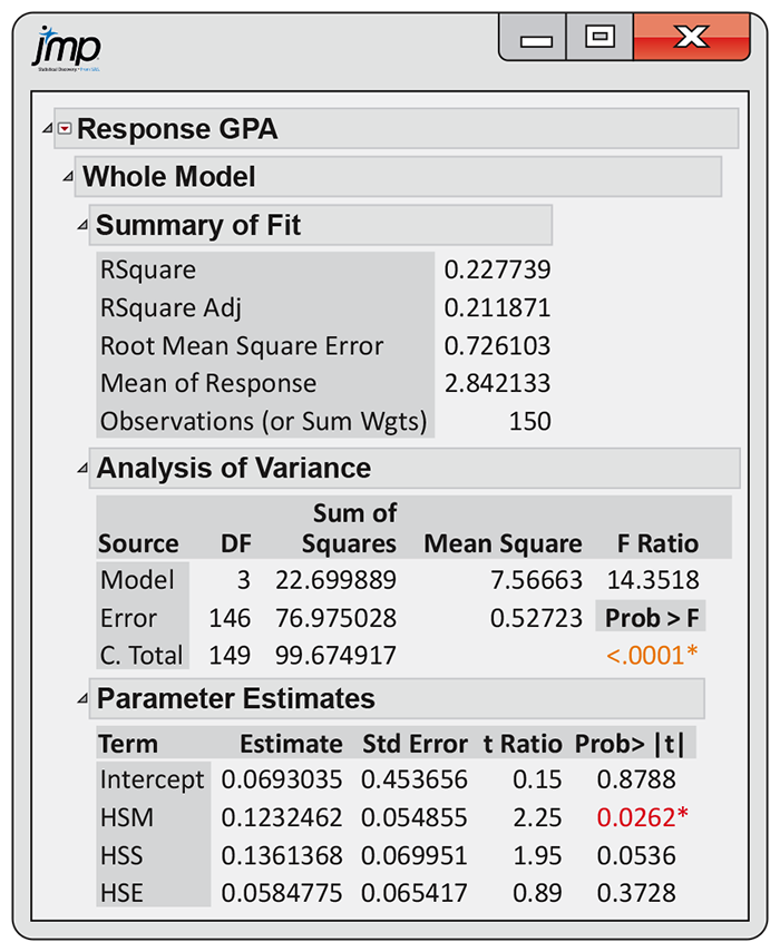
Figure 11.6 Multiple regression output for regression using high school grades to predict GPA, Example 11.6.
In the fit statistics that precede the ANOVA table, we find that
Root MSE is 0.726. This value is the square root of the MSE given in
the ANOVA table and is s, the estimate of the parameter
Although the P-value of the F test is very small, the model does not explain very much of the variation in GPA. Remember, a small P-value does not necessarily tell us that we have a strong predictive relationship, particularly when the sample size is large.
From the Parameter Estimates section of the output in Figure 11.6, we obtain the fitted regression equation
We can use this equation to predict the grade point average for any
incoming student. For example, if a student had an
Example 11.7 Regression on high school grades: The individual t tests.
![]()
The ANOVA F test assesses the predictive ability of the set of explanatory variables. It does not tell us if each variable is helpful, given the other variables in the model. That is assessed using the individual parameter t tests. These are also supplied in the Parameter Estimates section of Figure 11.6. Recall that the t statistics for testing the regression coefficients are obtained by dividing the estimates by their standard errors. Thus, for the coefficient of HSM, we obtain the t-value given in the output by calculating
The P-values appear in the last column. Note that these P-values are for the two-sided alternatives. HSM has a P-value of 0.0262, and we conclude that the regression coefficient for this explanatory variable is significantly different from 0. The P-values for the other explanatory variables (0.0536 for HSS and 0.3728 for HSE) do not achieve statistical significance.
Interpretation of results
The significance tests for the individual regression coefficients seem to contradict the impression obtained by examining the correlations in Figure 11.4. In that display, we see that the correlation between GPA and HSS is 0.44, and the correlation between GPA and HSE is 0.36. Both of these correlations are statistically significant, meaning that if we used HSS alone in a regression to predict GPA, or if we used HSE alone, we would obtain statistically significant regression coefficients.
This phenomenon is not unusual in multiple regression analysis. Part of the explanation lies in the correlations between HSM and the other two explanatory variables. These are rather high (at least compared with most other correlations in Figure 11.4). The correlation between HSM and HSS is 0.67, and that between HSM and HSE is 0.49. Thus, when we have a regression model that contains all three high school grades as explanatory variables, there is considerable overlap of the predictive information contained in these variables. This is called collinearity or multicollinearity. In extreme cases, collinearity can cause numerical instabilities that result in very imprecise parameter estimates.
As mentioned earlier,
![]() the significance tests for individual regression coefficients
assess the significance of each predictor variable, assuming that
all other predictors are included in the regression equation. Given that we use a model with HSM and HSS as predictors, the
coefficient of HSE is not statistically significant. Similarly, given
that we have HSM and HSE in the model, HSS does not have a significant
regression coefficient. HSM, however, adds significantly to our
ability to predict GPA even after HSS and HSE are already in the
model.
the significance tests for individual regression coefficients
assess the significance of each predictor variable, assuming that
all other predictors are included in the regression equation. Given that we use a model with HSM and HSS as predictors, the
coefficient of HSE is not statistically significant. Similarly, given
that we have HSM and HSE in the model, HSS does not have a significant
regression coefficient. HSM, however, adds significantly to our
ability to predict GPA even after HSS and HSE are already in the
model.
Unfortunately, we cannot conclude from this analysis that the pair of explanatory variables HSS and HSE contribute nothing significant to our model for predicting GPA once HSM is in the model. Questions like these require fitting additional models.
The impact of relationships among the several explanatory variables on fitting models for the response is the most important new phenomenon encountered in moving from simple linear regression to multiple regression. In this chapter, we can only illustrate some of the many complicated problems that can arise.
Examining the residuals
As in simple linear regression, we should always examine the residuals
as an aid to determining whether the multiple regression model is
appropriate for the data. Because there are several explanatory
variables, we must examine several residual plots. It is usual to plot
the residuals versus the predicted values
Example 11.8 Checking the Normality of the residuals.
If the deviations
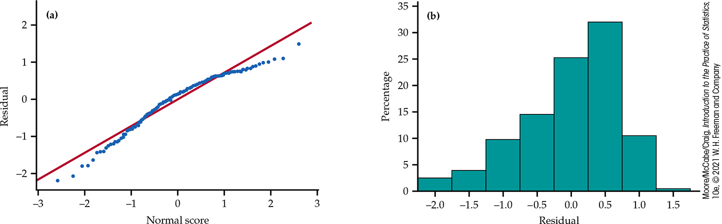
Figure 11.7 (a) Normal quantile plot and (b) histogram of the residuals from the high school grades model, Example 11.8.
When many observations are near this upper limit, inference can suffer from a ceiling effect. When the ceiling effect is too strong, least-squares regression can struggle to identify useful predictors and may lead to inaccurate predictions. Given the large sample size for this example, we do not think this skewness is strong enough to invalidate our inference on coefficients. This skewness, however, would be an issue if we considered constructing prediction intervals. More advanced models are available for analysis in the presence of a ceiling effect. Consult an expert if you are concerned that the effect may be too strong.
Check-in
-
11.5 Residual plots for the GPA analysis. Using a statistical package, fit the linear model with HSM, HSS, and HSE as predictors and obtain the residuals and predicted values. Plot the residuals versus the predicted values, HSM, HSS, and HSE. Are the residuals more or less randomly dispersed around zero? Comment on any unusual patterns.
Refining the model
Because the variable HSE has the largest P-value of the three explanatory variables (see Figure 11.6) and, therefore, appears to contribute the least to our explanation of GPA, we rerun the regression using only HSM and HSS as explanatory variables.
Example 11.9 Regression on HSM and HSS.
Minitab output appears in
Figure 11.8. The F statistic indicates that we can reject the null
hypothesis that the regression coefficients for the two explanatory
variables are both 0. The P-value is still
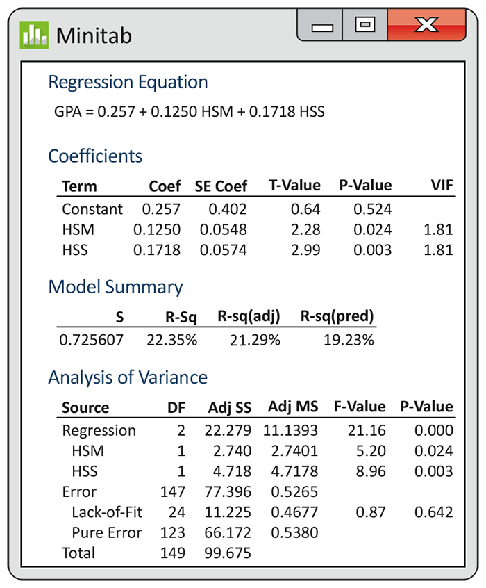
Figure 11.8 Multiple regression output for model using HSM and HSS to predict GPA, Example 11.9.
The estimated model standard deviation s is nearly identical
for the two regressions, which is another indication that we lose
very little when we drop HSE. The t statistics for the
individual regression coefficients indicate that HSM is still
significant
Comparison of the fitted equations for the two multiple regression analyses tells us something more about the intricacies of this procedure. For the first run, we have
whereas the second gives us
Eliminating HSE from the model changes the regression coefficients for
all the remaining variables and the intercept. This phenomenon occurs
quite generally in multiple regression.
![]() Individual regression coefficients, their standard errors, and
significance tests are meaningful only when interpreted in the
context of the other explanatory variables in the model.
Individual regression coefficients, their standard errors, and
significance tests are meaningful only when interpreted in the
context of the other explanatory variables in the model.
What should not change much if the two models have similar
The difference in estimates is small relative to the regression standard error.
Considering other sets of explanatory variables
Let’s now turn to the problem of predicting GPA using just the three SAT scores.
Example 11.10 Regression on SAT scores.
Figure 11.9 gives the Excel output for the multiple regression using the three SAT scores. The fitted model is
The degrees of freedom are as expected: 3, 146, and 149. The
F statistic is 6.28, with a P-value of 0.0005. We
conclude that the regression coefficients for SATM, SATCR, and SATW
are not all 0. Recall that we obtained the P-value
![]() Stating that we have a statistically significant result is quite
different from saying that an effect is large or important.
Stating that we have a statistically significant result is quite
different from saying that an effect is large or important.
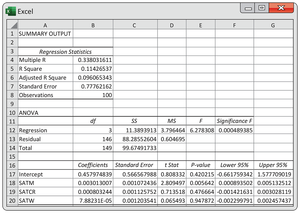
Figure 11.9 Multiple regression output for model using SAT scores to predict GPA, Example 11.10.
Further examination of the output in
Figure 11.9
reveals that the coefficient of SATM is significant
We have seen that fitting a model using either the high school grades
or the SAT scores results in a highly significant regression equation.
The mathematics component of each of these groups of explanatory
variables appears to be a key predictor. A comparison of the values of
Example 11.11 Regression using all variables.
To address this question, we run the regression with all six
explanatory variables. The output from JMP appears in
Figure 11.10. The degrees of freedom are as expected: 6, 143, and 149. The
F statistic is 8.95, with a P-value
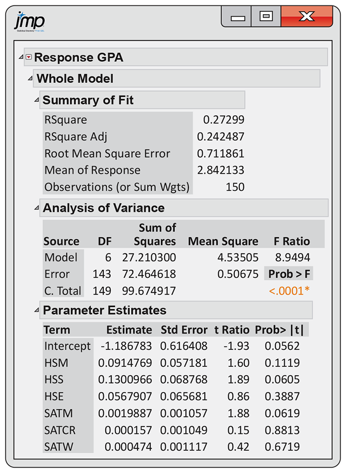
Figure 11.10 Multiple regression output for model using all variables to predict GPA, Example 11.11.
![]()
Examination of the t statistics and the associated P-values for the individual regression coefficients reveals a surprising result. None of the variables are significant! At first, this result may appear to contradict the ANOVA results. How can the model explain more than 27% of the variation and have t tests suggesting that none of the variables make significant contributions?
Once again, it is important to understand that these t tests assess the contribution of each variable when it is added to a model that already has the other five explanatory variables. This result does not necessarily mean that the regression coefficients for the six explanatory variables are all 0. It simply means that the contribution of each variable overlaps considerably with the contributions of the other five variables already in the model.
When a model has a large number of insignificant variables, it is common to refine the model. This is often termed model selection. We prefer smaller models to larger models because they are easier to work with and understand. However, given the many complications that can arise in multiple regression, there is no universal “best” approach to refine a model. There is also no guarantee that there is just one acceptable refined model.
Many statistical software packages now provide the capability of
summarizing all
Figure 11.11
contains Minitab output that shows the two best models in terms of
highest
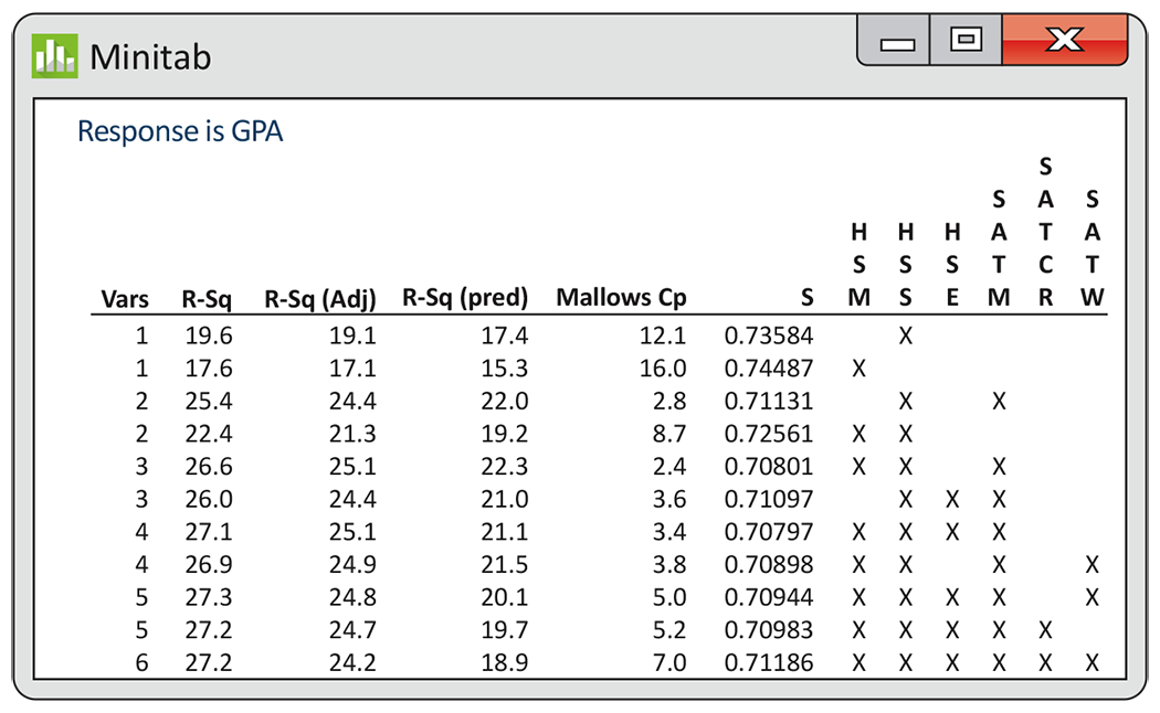
Figure 11.11 Minitab output, summarizing the fit of different regression models based on several model selection methods.
The list also contains the regression standard error s. Finding
a model (or models) that minimizes this quantity is another model
selection approach. It is equivalent to choosing a model based on the
largest
adjusted
Test for a collection of regression coefficients
Many statistical software packages also provide the capability for testing whether a collection of regression coefficients in a multiple regression model are all 0. We use this approach to address two interesting questions about our GPA data set. We did not discuss such tests in the first section of this chapter, but the basic idea is quite simple and is discussed in Exercise 11.30 (page 591).
In the context of the multiple regression model with all six predictors, we ask first whether or not the coefficients for the three SAT scores are all 0. In other words, do the SAT scores add any significant predictive information to that already contained in the high school grades? To be fair, we also ask the complementary question: Do the high school grades add any significant predictive information to that already contained in the SAT scores?
The answers are given in the R output in
Figure 11.12. For the first test, we see that
The test statistic for the three high school grade variables is
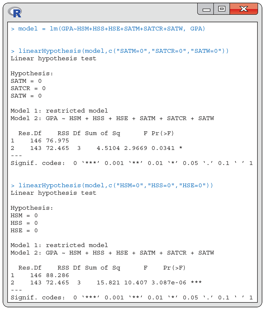
Figure 11.12 R output, summarizing two tests for different collections of regression coefficients.
Section 11.2 SUMMARY
- Multiple linear regression should always begin with a careful examination of the data. This involves looking at each variable separately and then at pairs of variables. Cases with extreme values should be noted and examined carefully throughout the analysis.
- Multiple linear regression has the same model conditions as simple linear regression. Prior to inference, always examine the distribution of the residuals and plot the residuals against each of the explanatory variables to make sure there are no remaining patterns and to ensure that there is constant variance.
-
The estimate
-
When p is large, consider using
model selection methods such as
adjusted
Section 11.2 EXERCISES
-
11.21 Annual ranking of world universities. Since 2004, Times Higher Education has provided an annual ranking of the world universities.6 A total score for each university is calculated based on weighting the scores for the following five categories: Teaching (30%), Research (30%), Citations (30%), Industry Income (2.5%), and International Outlook (7.5%). Assuming that we don’t know these weights, let’s consider developing a model to predict total score (Overall) based on a sample of 50 universities and using only the first three category scores: Teaching, Research, and Citations.

-
Using numerical and graphical summaries, describe the distribution of each explanatory variable.
-
Using numerical and graphical summaries, describe the relationship between each pair of explanatory variables.
-
-
11.22 Looking at the simple linear regressions. Refer to the previous exercise. Now look at the relationship between each explanatory variable and the total score.
-
Generate scatterplots for each explanatory variable and the total score. Do these relationships all look linear?
-
Compute the correlation between each explanatory variable and the total score. Are certain explanatory variables more strongly associated with the total score than others?
-
-
11.23 Multiple linear regression model. Refer to the previous two exercises. Let’s now consider a linear regression using all three explanatory variables.
-
Write out the statistical model for this analysis, making sure to specify all assumptions.
-
Run the multiple regression model and specify the fitted regression equation.
-
Obtain the residuals and check the conditions needed for inference.
-
Generate a 95% confidence interval for each coefficient. Explain what these intervals tell you.
-
What percent of the variation in total score is explained by this model? What is the estimate for
-
-
11.24 Explaining the results. Refer to the previous exercise. A friend, knowing that these three categories were all weighted the same by Times Higher Education, does not understand why your model fit seems to suggest different weights for these three scores. Explain to your friend why this can happen.
-
11.25 Refining the GPA model: Residual checks. Figure 11.11 (page 574) provides a list of the top models based on
-
11.26 Considering a transformation. When we regressed GPA versus the high school scores, the residuals were skewed to the left (Figure 11.7, page 583). Refit the model but now use
-
11.27 Refining the GPA model: Inference. Refer to Exercise 11.25. For each of the four models under consideration, report the least-squares equation, estimated model standard deviation s, and P-values for each of the individual coefficients. Based on these results and the residuals checks of the previous exercise, which model do you think is most preferred? Explain your answer.
-
11.28 Predicting college debt: Multiple regression. Refer to Exercises 10.6 (page 536) and 10.11 (page 537) for a description of the problem and data set. Let’s now consider fitting a model to predict average debt (AveDebt) using all four explanatory variables: Admit, Grad4Rate, InCost, and InCostAid.

-
Write out the statistical model for this analysis, making sure to specify all assumptions.
-
Run the multiple regression model and specify the fitted regression equation.
-
Obtain the residuals from part (b) and check assumptions. Is Colorado School of Mines still an unusual case? Or can we proceed with inference using the entire data set? Provide a brief summary.
-
-
11.29 Predicting college debt: Inference. Refer to the previous exercise. Let’s proceed using the entire data set.
-
Report the F statistic, its degrees of freedom, and the P-value. What do you conclude based on this test result?
-
What percent of the variability in average debt is explained by this model?
-
Using this F test and the individual parameter t tests, write a one-paragraph summary of this model’s fit to the data.
-
-
11.30 Testing a collection of variables. Refer to the previous exercise. Although the F test was highly significant, only Admit is found to be significant using the individual parameter t tests. This raises the question whether the other three variables further contribute to the prediction of average debt, given that the admittance rate is in the model.
In this chapter, we discussed the F test for a collection of regression coefficients. In most cases, this capability is provided by the software. When it is not, the test can be performed using the
with q and
-
11.31 A mechanistic explanation of popularity. In Exercise 10.61 (page 561), correlations between an adolescent’s “popularity,” expression of a serotonin receptor gene, and rule-breaking behaviors were assessed. An additional portion of the analysis looked at the relationship between the gene expression level and popularity, after adjusting for rule-breaking (RB) behaviors. This adjustment was necessary because RB is positively associated both with this gene expression and with popularity in adolescents. The following table summarizes these regression analyses using the composite (questionnaire and video) RB score. A total of 202 individuals were included in this analysis.
b s(b) Model 1 Gene expression 0.204 0.066 Model 2 Gene expression 0.161 0.066 RB.composite 0.100 0.030 For all analyses, use the 0.05 significance level.
-
What are the error degrees of freedom for Model 1 and for Model 2?
-
Test the null hypothesis that the serotonin gene receptor coefficient is equal to 0 in Model 1. State the test statistic and P-value.
-
Perform both individual-variable t tests for Model 2. Again state the test statistics and P-values.
-
Is there still a positive relationship between the serotonin gene receptor expression level and popularity, after adjusting for RB? If yes, compare the increase in popularity for a unit increase in gene expression (while RB remains unchanged) in the two models.
-
-
11.32 Consider the sex of the students. Refer to Example 11.11 (page 586). The seventh explanatory variable provided in the GPA data set is a sex indicator variable. This variable (Sex) takes the value 0 for males and 1 for females. If we include it in our model involving the other six variables, it allows the intercept to differ for the two sexes (see Exercises 11.16 and 11.17, pages 574 and 575).
-
Include the variable Sex with the other six explanatory variables and refit the model. Compare the fit of this model, using
-
Does this indicator variable appear to contribute to our explanation of GPA? Report the test results.
-
Does the coefficient suggest that males or females have higher GPA scores? Explain your answer.
-
-
11.33 Predicting energy-drink consumption. Energy-drink advertising consistently emphasizes a physically active lifestyle and often features extreme sports and risk taking. Are these typical characteristics of an energy-drink consumer? A researcher decided to examine the links between energy-drink consumption, sport-related (jock) identity, and risk taking.7 She invited more than 1500 undergraduate students enrolled in large introductory-level courses at a public university to participate. Each participant had to complete a 45-minute anonymous questionnaire. From this questionnaire, jock identity and risk-taking scores were obtained, where the higher the score, the stronger the trait. She ended up with 795 respondents. The following table summarizes the results of a multiple regression analysis using the frequency of energy-drink consumption in the past 30 days as the response variable:
Explanatory variable b Age Sex Race Ethnicity 0.10** Parental education 0.02 College GPA Jock identity 0.05 Risk taking 0.19*** The superscript ** means that the individual coefficient t test had a P-value less than 0.01, and the superscript *** means that the test had a P-value less than 0.001. All other P-values were greater than 0.05.
-
The overall F statistic is reported to be 8.11. What are the degrees of freedom associated with this statistic?
-
R is reported to be 0.28. What percent of the variation in energy-drink consumption is explained by the model? Is this a highly predictive model? Explain.
-
Interpret each of the regression coefficients that are significant.
-
The researcher states, “Controlling for gender, age, race, ethnicity, parental educational achievement, and college GPA, each of the predictors (risk taking and jock identity) was positively associated with energy-drink consumption frequency.” Explain what is meant by “controlling for” these variables and how this helps strengthen her assertion that jock identity and risk taking are positively associated with energy-drink consumption.
-
-
11.34 Is the number of tornadoes increasing? In Exercise 10.15, data on the number of tornadoes in the United States between 1953 and 2019 were analyzed to see if there was a linear trend over time. Some argue that it’s not the number of tornadoes increasing over time but rather the probability of sighting them is increasing because there are more people living in the United States. Let’s investigate this by including the U.S. census count as an additional explanatory variable.

-
Using numerical and graphical summaries, describe the relationship between each pair of variables.
-
Perform a multiple regression using both year and census count as explanatory variables. Write down the fitted model.
-
Obtain the residuals from part (b). Plot them versus the two explanatory variables and generate a Normal quantile plot. What do you conclude?
-
Test the hypothesis that there is a linear increase over time. State the null and alternative hypotheses, test statistic, and P-value. What is your conclusion?
-